Literature on implementing a Zero-Inflated Beta likelihood

I was wondering if there were any specific examples of modeling a mixture process where one process produces 0’s and the other follows a beta distribution.

I know that there exists ZeroInflated distributions in the library and I can use the base Beta distribution to implement one myself, but I was wondering if this would be the preferred way of handling such a process.

Any help would be appreciated.

2 Likes

I don’t know any such example. I think it would be very difficult, as the Beta distribution support does not include neither 0 nor 1. Your mixture’s logp would have to deal very carefully with infs and your random method would also have to handle domain errors.

To work around this, I am imputing the 0’s with a small epsilon, say 1e-3, logit transforming the data, and saying the likelihood is a Normal distribution of the logit transformed data. I can then say that if data is at or below 1e-3 then we treat as 0 in the zero inflated model otherwise follow the normal likelihood.

Would there be someway of incorporating that into a Mixture model or subclassing the Normal distribution to deal with the multi-modality?

You could try to write down a mixture of a Beta and a Uniform(0, 1e-3) in this case. The logit transform could also use a similar kind of mixture approach. I’m not really familiar with censored models, but this problem sounds like it could be addressed with a censored model

Hmm, could you give an example of such a mixture or would someone else be able to?

Thanks for the response!

Yes, it would look something like this

with pm.Model():
    w = pm.Beta('w', 1, 1)
    alpha = pm.HalfNormal('alpha', 1)
    beta = pm.HalfNormal('beta', 1)
    mixture_beta = pm.Beta('mixb', alpha, beta)
    u = pm.Uniform('u', 0, 1e-3)
    mixture = pm.Mixture('mixture', [w, 1-w],
                 comp_dists=[mixture_beta.distribution, u.distribution])
2 Likes

You need to pass a vector for w and distribution for comp_dists:

mixture = pm.Mixture('mixture', 
                     [w, 1-w], 
                     comp_dists=[mixture_beta.distribution, 
                                 u.distribution])
3 Likes

You’re right! I’ve edited my example code with your correction

Thank you very much for the example. @junpenglao, do you have any experience with a censored model implementation? That actually sounds simpler and more like what I need.

Also, in the docs for the Mixture class, shouldn’t the support of the mixture be \bigcup_{i=0}^n \text{support}(f_i) not \bigcap_{i=0}^n \text{support}(f_i)?

https://docs.pymc.io/api/distributions/mixture.html#pymc3.distributions.mixture.Mixturez

Lastly, the above snippet will not sample. I changed the prior for the Beta parameters to be uniform(1, 10) to test it out but an error is raised stating bad initial energy.

The bad initial energy could be caused by many reasons. I think that it may have to do with the upper boundary of the Uniform distribution being equal to the imputed variable 1e-3. This makes the uniform always return -\infty and makes the model try to get w=1, which is imposible. Maybe if you just impute with values that are truly random and taken from a uniform with lower 0 and upper 1 bounds you will be able to sample. You could also change the upper boundary of the imputation uniform distribution to 2e-3.

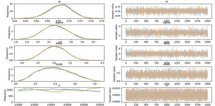
I wrote a more self contained example that generates the observed data using the model, then samples and then plots the trace and posterior predictives, and everything works:

import numpy as np
import pymc3 as pm
from matplotlib import pyplot as plt


def model_factory(observed=None, generate=False, true_parameters=None,
                  nsamples=500, *args, **kwargs):
    with pm.Model(*args, **kwargs) as model:
        w = pm.Beta('w', 1, 1)
        alpha = pm.HalfNormal('alpha', 1)
        beta = pm.HalfNormal('beta', 1)
        mixture_beta = pm.Beta('mixb', alpha, beta)
        u = pm.Uniform('u', 0, 1e-3)
        if observed is None:
            mixture = pm.Mixture('mixture', [w, 1-w],
                                 comp_dists=[mixture_beta.distribution,
                                             u.distribution])
        else:
            mixture = pm.Mixture('mixture', [w, 1-w],
                                 comp_dists=[mixture_beta.distribution,
                                             u.distribution],
                                 observed=observed)
        if generate:
            if true_parameters is None:
                true_parameters = {}
            generated_data = mixture.random(point=true_parameters,
                                            size=nsamples)
            return model, generated_data
        else:
            return model


observed = model_factory(generate=True,
                         true_parameters={'w': np.array(0.7),
                                          'alpha': np.array(4),
                                          'beta': np.array(6),
                                          })[1]
with model_factory(observed=observed) as model:
    trace = pm.sample(2000, tune=1000)
    pm.traceplot(trace)
    plt.figure()
    ppc = pm.sample_posterior_predictive(trace)
    plt.hist(observed, 50, histtype='step', color='b')
    for mix in ppc['mixture'][::100]:
        plt.hist(mix, 50, histtype='step',
                 color='r', alpha=0.05)

The traceplot returns

And the posterior predictive looks like this:
mixture_ppc

1 Like

This is fantastic and is much appreciated! Thank you!

I have been trying to recreate the above model construction using my own construct_model function that makes use of a design matrix of shape (M, N) and observed data of shape (M, 1). Unfortunately, naively taking the above code and inserting the weights and mixture distribution results in the following error:

---------------------------------------------------------------------------
AttributeError                            Traceback (most recent call last)
/anaconda3/envs/audience-concentration-forecast-service-env/lib/python3.6/site-packages/pymc3/distributions/mixture.py in _comp_means(self)
    119         try:
--> 120             return tt.as_tensor_variable(self.comp_dists.mean)
    121         except AttributeError:

AttributeError: 'list' object has no attribute 'mean'

During handling of the above exception, another exception occurred:

IndexError                                Traceback (most recent call last)
<ipython-input-18-69ac3b7b6842> in <module>
----> 1 model = construct_model(data, preprocessors)

<ipython-input-17-51f9055e6674> in construct_model(data, preprocessors, fit_intercept)
     63                              w=[weights, 1 - weights],
     64                              comp_dists=[measured.distribution, unmeasured.distribution],
---> 65                              observed=success_rate)
     66 
     67     return model

/anaconda3/envs/audience-concentration-forecast-service-env/lib/python3.6/site-packages/pymc3/distributions/distribution.py in __new__(cls, name, *args, **kwargs)
     39                 raise TypeError("observed needs to be data but got: {}".format(type(data)))
     40             total_size = kwargs.pop('total_size', None)
---> 41             dist = cls.dist(*args, **kwargs)
     42             return model.Var(name, dist, data, total_size)
     43         else:

/anaconda3/envs/audience-concentration-forecast-service-env/lib/python3.6/site-packages/pymc3/distributions/distribution.py in dist(cls, *args, **kwargs)
     50     def dist(cls, *args, **kwargs):
     51         dist = object.__new__(cls)
---> 52         dist.__init__(*args, **kwargs)
     53         return dist
     54 

/anaconda3/envs/audience-concentration-forecast-service-env/lib/python3.6/site-packages/pymc3/distributions/mixture.py in __init__(self, w, comp_dists, *args, **kwargs)
     84 
     85             try:
---> 86                 self.mean = (w * self._comp_means()).sum(axis=-1)
     87 
     88                 if 'mean' not in defaults:

/anaconda3/envs/audience-concentration-forecast-service-env/lib/python3.6/site-packages/pymc3/distributions/mixture.py in _comp_means(self)
    122             return tt.squeeze(tt.stack([comp_dist.mean
    123                                         for comp_dist in self.comp_dists],
--> 124                                        axis=1))
    125 
    126     def _comp_modes(self):

/anaconda3/envs/audience-concentration-forecast-service-env/lib/python3.6/site-packages/theano/tensor/basic.py in stack(*tensors, **kwargs)
   4707         dtype = scal.upcast(*[i.dtype for i in tensors])
   4708         return theano.tensor.opt.MakeVector(dtype)(*tensors)
-> 4709     return join(axis, *[shape_padaxis(t, axis) for t in tensors])
   4710 
   4711 

/anaconda3/envs/audience-concentration-forecast-service-env/lib/python3.6/site-packages/theano/tensor/basic.py in <listcomp>(.0)
   4707         dtype = scal.upcast(*[i.dtype for i in tensors])
   4708         return theano.tensor.opt.MakeVector(dtype)(*tensors)
-> 4709     return join(axis, *[shape_padaxis(t, axis) for t in tensors])
   4710 
   4711 

/anaconda3/envs/audience-concentration-forecast-service-env/lib/python3.6/site-packages/theano/tensor/basic.py in shape_padaxis(t, axis)
   4599     if not -ndim <= axis < ndim:
   4600         msg = 'axis {0} is out of bounds [-{1}, {1})'.format(axis, ndim)
-> 4601         raise IndexError(msg)
   4602     if axis < 0:
   4603         axis += ndim

IndexError: axis 1 is out of bounds [-1, 1)

The snippet below abstractly constructs the model:

import logging
import numpy as np
import pymc3 as pm
import scipy.sparse
import theano


def assemble_coefficient_vector(feature_shapes, default_sd=2.5):
    """Using the dictionary of features and their dimensions (shapes), assemble
    the coefficient vector to be used for regression. We assume that the design_matrix
    does not contain a vector of 1's for the intercept.
    """
    coefficient_vector = []

    for feature in feature_shapes:
        # Get number of features
        N = feature_shapes[feature]

        sigma = pm.HalfStudentT(f'σ_{feature}', nu=4, sd=default_sd)
        coefficients = pm.StudentT(f'β_{feature}', nu=4, mu=0, sd=sigma, shape=(N, 1))

        coefficient_vector.append(coefficients)

    coefficient_vector = theano.tensor.concatenate(coefficient_vector, axis=0)

    return coefficient_vector


def construct_model(data, preprocessors):
    # create model just relies on preprocessors (design_matrix, response) and data
    design_matrix_preprocessor = preprocessors['design_matrix']
    response_preprocessor = preprocessors['response']

    feature_shapes = mp.get_feature_shapes(design_matrix_preprocessor)

    design_matrix = design_matrix_preprocessor.transform(data)
    M, N = design_matrix.shape

    response = response_preprocessor.transform(data)

    X = theano.sparse.as_sparse_variable(design_matrix)
    success_rate = theano.tensor.as_tensor_variable(response)

    with pm.Model() as model:
        # Of shape (N, 1)
        coefficient_vector = assemble_coefficient_vector(feature_shapes, fit_intercept=fit_intercept)

        # Multiply matrix M x N times vector N x 1 to get M x 1 vector
        mu = theano.sparse.dot(X, coefficient_vector)
        kappa = pm.HalfStudentT('κ', sd=2.5)

        likelihood = pm.StudentT('likelihood', nu=4, mu=mu, sd=kappa, observed=success_rate)

    return model

Is there something obviously wrong that I am doing?

And sorry, this is the construct_model definition with the modifications:

def construct_model(data, preprocessors, fit_intercept=False):
    # create model just relies on preprocessors (design_matrix, response) and data
    design_matrix_preprocessor = preprocessors['design_matrix']
    response_preprocessor = preprocessors['response']

    ZERO = float(response_preprocessor.transform(pd.DataFrame({'success_rate': [0.0]})))
    ONE = float(response_preprocessor.transform(pd.DataFrame({'success_rate': [1.0]})))

    feature_shapes = mp.get_feature_shapes(design_matrix_preprocessor)

    design_matrix = design_matrix_preprocessor.transform(data)
    M, N = design_matrix.shape

    # Add a vector of ones to first column of design_matrix.
    if fit_intercept:
        intercept_design_matrix = np.concatenate([np.ones(shape=(M, 1)), design_matrix.todense()], axis=1)
        design_matrix = scipy.sparse.csr_matrix(intercept_design_matrix)

    response = response_preprocessor.transform(data)

    X = theano.sparse.as_sparse_variable(design_matrix)
    success_rate = theano.tensor.as_tensor_variable(response)

    with pm.Model() as model:
        weights = pm.Beta('w', 1, 1)

        coefficient_vector = assemble_coefficient_vector(feature_shapes, fit_intercept=fit_intercept)

        mu = theano.sparse.dot(X, coefficient_vector)
        kappa = pm.HalfStudentT('κ', nu=4, sd=2.5)

        measured = pm.StudentT('measured', nu=4, mu=mu, sd=kappa, shape=(M, 1))

        unmeasured = pm.Normal('unmeasured', mu=ZERO, sd=1e-3, shape=(M, 1))

        mixture = pm.Mixture('mixture', 
                             w=[weights, 1 - weights], 
                             comp_dists=[measured.distribution, unmeasured.distribution],
                             observed=success_rate)

    return model
Here is a histogram of a typical proportion dataset that I am trying to describe:

image

and here is the standardized logit transform of the above proportion data:

image

The logit transform data is what I am trying to fit to a Student T distribution and would like to describe the “zero” generating process somehow. Some sort of “zero inflated normal/student t distribution” would suffice.

This probably isn’t useful, but I was able to get the Mixture likelihood with (M, 1) vectors through the following code:

import numpy as np
import scipy
import theano.tensor as tt

M = 100
process_1_rate = 0.25

process_1 = scipy.stats.norm.rvs(loc=-2, scale=1, size=100)
process_2 = scipy.stats.norm.rvs(loc=2, scale=1, size=100)

coinflips = np.random.random(size=M)

process_1_index = np.where(coinflips <= process_1_rate)[0]
process_2_index = np.array(list(set(range(M)).difference(set(process_1_index))))

observed = np.concatenate([process_1[process_1_index], process_2[process_2_index]])
observed = observed.reshape(-1, 1)


with pm.Model():
    mixture_1 = pm.Normal.dist(mu=-2, sd=1, shape=(M, 1))
    mixture_2 = pm.Normal.dist(mu=2, sd=1, shape=(M, 1))

    w = pm.Dirichlet('w', a=np.array([1, 1]))

    like = pm.Mixture('like', w=w, comp_dists=[mixture_1, mixture_2], observed=tt.as_tensor_variable(observed))

    trace = pm.sample()
    pm.traceplot(trace)
    plt.show()

I’m just confused as to why the code posted previously is failing when it’s very similar to this snippet.

The assemble_coefficient_vector seems to have an error. Where you wrote:

        coefficients = pm.StudentT(f'β_{feature}', nu=4, mu=0, sd=sigma, shape=(N, 1))

        coefficient_vector.append(coefficients)

    coefficient_vector = theano.tensor.concatenate(coefficient_vector, axis=0)

The coefficients random variable is a 2D array of shape (N, 1). Then when you concatenate, you are doing so on axis=0, which means that the output’s shape will be (M*N, 1). You should change those lines to:

        coefficients = pm.StudentT(f'β_{feature}', nu=4, mu=0, sd=sigma, shape=(N,))

        coefficient_vector.append(coefficients)

    coefficient_vector = theano.tensor.stack(coefficient_vector)

Checkout stack's documentation and you’ll see that this will output an (M, N) shaped tensor.

Sorry, I should have been more clear:

the feature_shapes variable is a dictionary of key-value pairs that are features-number of covariates, e.g.

feature_shapes = {'feature_1': n_1, 'feature_2': n_2, ..., 'feature_k': n_k} 

where \sum_{i=1}^k n_k = N, which is the number of columns in the design_matrix X. Thus, I think we do want the coefficient vector to be N x 1 so that when we multiply it with the M x N design matrix we get the M x 1 vector to use as the mean of the likelihood.

I think the issue with the mixture class is that the mu variable of the StudentT distribution is a vector which is causing the issue. I’m not sure how to get around this though.

The code snippet below illustrates the same issue I am facing.

import numpy as np
import scipy
import theano.tensor as tt

M = 100
process_1_rate = 0.25

process_1 = scipy.stats.norm.rvs(loc=-2, scale=1, size=100)
process_2 = scipy.stats.norm.rvs(loc=2, scale=1, size=100)

coinflips = np.random.random(size=M)

process_1_index = np.where(coinflips <= process_1_rate)[0]
process_2_index = np.array(list(set(range(M)).difference(set(process_1_index))))

observed = np.concatenate([process_1[process_1_index], process_2[process_2_index]])
observed = observed.reshape(-1, 1)

with pm.Model():
    mu_1 = pm.Normal('mu_1', mu=-1, sd=2, shape=(M, 1))
    mu_2 = pm.Normal('mu_2', mu=1, sd=2, shape=(M, 1))

    sd_1 = pm.HalfNormal('sd_1', sd=1, shape=(1, 1))
    sd_2 = pm.HalfNormal('sd_2', sd=1, shape=(1, 1))

    mixture_1 = pm.Normal.dist(mu=mu_1, sd=sd_1)
    mixture_2 = pm.Normal.dist(mu=mu_2, sd=sd_2)

    w = pm.Dirichlet('w', a=np.array([1, 1]))

    like = pm.Mixture('like', w=w, comp_dists=[mixture_1, mixture_2], 
                                observed=tt.as_tensor_variable(observed))

Particularly, when the Mixture class tries to obtain the mean it executes

tt.squeeze(tt.stack([comp_dist.mean for comp_dist in self.comp_dists], axis=1)) 

and I am getting the dimension error mentioned above.

I see… Could you post this last snippet as an issue on github? We’ll take a closer look at it, but it looks like another one of our beloved shape problems.

I actually can’t reproduce your error with the code snippet you provided

import numpy as np
import scipy
import theano.tensor as tt
import pymc3 as pm
from matplotlib import pyplot as plt

M = 100
process_1_rate = 0.25

process_1 = scipy.stats.norm.rvs(loc=-2, scale=1, size=100)
process_2 = scipy.stats.norm.rvs(loc=2, scale=1, size=100)

coinflips = np.random.random(size=M)

process_1_index = np.where(coinflips <= process_1_rate)[0]
process_2_index = np.array(list(set(range(M)).difference(set(process_1_index))))

observed = np.concatenate([process_1[process_1_index],
                           process_2[process_2_index]])
observed = observed.reshape(-1, 1)

with pm.Model():
    mu_1 = pm.Normal('mu_1', mu=-1, sd=2, shape=(M, 1))
    mu_2 = pm.Normal('mu_2', mu=1, sd=2, shape=(M, 1))

    sd_1 = pm.HalfNormal('sd_1', sd=1, shape=(1, 1))
    sd_2 = pm.HalfNormal('sd_2', sd=1, shape=(1, 1))

    mixture_1 = pm.Normal.dist(mu=mu_1, sd=sd_1) # The mixture random is faster if shape is provided here
    mixture_2 = pm.Normal.dist(mu=mu_2, sd=sd_2) # The mixture random is faster if shape is provided here

    w = pm.Dirichlet('w', a=np.array([1, 1]))

    like = pm.Mixture('like', w=w, comp_dists=[mixture_1, mixture_2],
                      observed=tt.as_tensor_variable(observed))
    prior = pm.sample_prior_predictive()
    trace = pm.sample()
    ppc = pm.sample_posterior_predictive(trace)

    pm.traceplot(trace)
    plt.hist(observed, 50, histtype='step', color='b')
    for mix in ppc['like'][::20]:
        plt.hist(mix, 50, histtype='step',
                 color='r', alpha=0.05)

The model samples (although it is super divergent)


mixture2_ppc

1 Like

Hi @lucianopaz,

It appears you are right. I must have changed something unintentionally that made it work and didn’t notice.

I’m not even sure I wrote that model to do what I thought it did which was to associate a weight to each record of belonging in one class over the other.