DISCLAIMER
This is a repost of a CrossValidated question which has got no answers till now.
Goal
My goal is to perform a bayesian A/B test of probabilities of success in two groups considering a hypothesis about non-zero covariance between those probabilities.
Bivariate beta distribution
I am trying to implement a bivariate beta distribution model as proposed by Barry C.Arnold, Hon Keung Tony Ng in “Flexible bivariate beta distributions” using PyMC3. The main formulae is denoted (1) in the article:
Bivariate random variable (X, Y) is defined as a function of five Gamma distributed variables U_i with scale parameters equal to 1:
U_i \sim Gamma(\alpha_i, 1)
X = \frac{U_1+U_3}{U_1+U_3+U_4+U_5}; Y = \frac{U_2+U_4}{U_2+U_3+U_4+U_5}
When constructed this way, random variables (X, Y) are meant to present a (possibly) covariated pair of Beta random variables.
The marginal distributions of X and Y are beta distributions with parameters (\alpha_1+\alpha_3, \alpha_4+\alpha_5) and (\alpha_2+\alpha_4, \alpha_3+\alpha_5), respectively.
Data
I have a small (generated) dataset containing daily numbers of trials (denoted trials_a and trials_b) and successes (denoted successes_a and successes_b) in two groups (a/b testing). Daily conversion rates are correlated and I’d like to take that fact into account while sampling from posterior beta distributions to obtain more relevant estimation of difference between conversion rates.
Also I have some prior knowledge about marginal betas, e.g. from analyzing data obtained before the start of a/b test. Let’s consider prior_alpha=20 and prior_beta=4980 which are equal for both marginals.
The code in python for generating a dataset is as following:
from scipy import stats
import numpy as np
import pandas as pd


DAYS = 30

# params for generating daily number of trials
TRIALS_MEAN = 5000
TRIALS_STD = 200**2
TRIALS_COV_FACTOR = 0.999

# prior knowledge about probability of success in both groups
PRIOR_ALPHA = 20
PRIOR_BETA = TRIALS_MEAN - PRIOR_ALPHA

# (unknown) probability of success in group A should be a little less than in prior
PROB_A_ALPHA = PRIOR_ALPHA - 1
PROB_A_BETA = TRIALS_MEAN - PROB_A_ALPHA

# (unknown) probability of success in group B should be a little more than in prior
PROB_B_ALPHA = PRIOR_ALPHA + 1
PROB_B_BETA = TRIALS_MEAN - PROB_B_ALPHA

# some value which allows covariance in probabilities via normal copula
BETAS_COPULA_COV_FACTOR = 0.5

np.random.seed(0)


def make_data():
    def make_trials():
        """Creates strongly correlated daily number of trials"""
        mvnorm = stats.multivariate_normal(
            mean=[TRIALS_MEAN, TRIALS_MEAN],
            cov=[[TRIALS_STD, TRIALS_COV_FACTOR*TRIALS_STD],
                 [TRIALS_COV_FACTOR*TRIALS_STD, TRIALS_STD]])
        return mvnorm.rvs(DAYS).astype(int)

    def make_probs():
        """Creates correlated daily probs of success using normal copula"""

        def covariate(rv1: stats.rv_continuous, rv2: stats.rv_continuous, cov_factor: float, n: int):
            def make_copula():
                mvnorm = stats.multivariate_normal(mean=[0, 0], cov=[[1., cov_factor],
                                                                     [cov_factor, 1.]])
                # Generate random samples from multivariate normal with covariance
                x = mvnorm.rvs(n)
                return stats.norm.cdf(x=x)

            copula = make_copula()
            s1 = rv1.ppf(copula[:, 0])
            s2 = rv2.ppf(copula[:, 1])
            return np.vstack((s1, s2))

        beta_a = stats.beta(PROB_A_ALPHA, PROB_A_BETA)
        beta_b = stats.beta(PROB_B_ALPHA, PROB_B_BETA)
        return covariate(rv1=beta_a, rv2=beta_b, cov_factor=BETAS_COPULA_COV_FACTOR, n=DAYS).T

    trials = make_trials()
    probs = make_probs()
    # creates daily number of successes by sampling from binomial with corresponding number of trials
    # and prob of success

    successes = np.random.binomial(trials, probs)

    df = pd.DataFrame(
        np.hstack(
            (trials, probs, successes)
        ),
        columns=['trials_a', 'trials_b', 'prob_a', 'prob_b', 'successes_a', 'successes_b']
    )
    return df


df = make_data()
print(df.head())
# output:
#   trials_a  trials_b    prob_a    prob_b  successes_a  successes_b
#0    4645.0    4649.0  0.004429  0.004510         15.0         28.0
#1    4794.0    4814.0  0.005251  0.003992         28.0         34.0
#2    4630.0    4622.0  0.003775  0.003821         13.0         22.0
#3    4810.0    4809.0  0.004845  0.005806         19.0         29.0
#4    5018.0    5022.0  0.004427  0.004914         17.0         30.0
Model in theory
As mentioned above, I have some prior knowledge about the marginal distributions of betas:
X_{margin} = Y_{margin} = Beta(prior\_alpha, prior\_beta)
And we have their expressions in terms of \alpha_i from the paper:
X_{margin} = Beta(\alpha_1+\alpha_3, \alpha_4+\alpha_5); Y_{margin} = Beta(\alpha_2+\alpha_4, \alpha_3+\alpha_5)
Unfortunately I don’t know anything about covariance prior. Therefore my prior knowledge about \alpha s can be expressed like this (I am very unsure about correctness of these lines):
some\_latent\_var = Uniform(0.001, min(prior\_alpha, prior\_beta))
\alpha_3, \alpha_4 \sim some\_latent\_var
\alpha_1, \alpha_2 \sim prior\_alpha - some\_latent\_var
\alpha_5 \sim prior\_beta - some\_latent\_var
So then I incorporate the model mentioned above:
U_i \sim Gamma(\alpha_i, 1)
X = \frac{U_1+U_3}{U_1+U_3+U_4+U_5}; Y = \frac{U_2+U_4}{U_2+U_3+U_4+U_5}
And finally in test groups a and b I have N (N = 30 in the example) independent and identically distributed binomial variables which generate daily number of succeses from daily number of trials (the latter are considered to be non-random). Probability of success in groups a and b follow the X and Y distributions respectively. Denoting day d's and group k's number of trials trials_{k, d} and number of successes successes_{k, d}:
\forall d \in [1, N]: successes_{a, d} \sim Binomial(trials_{a, d}, X)
\forall d \in [1, N]: successes_{b, d} \sim Binomial(trials_{b, d}, Y)
I have both successes and trials in both groups in my dataset. Therefore I can construct this model in PyMC3 and sample from it to obtain posteriors for X and Y.
Model in practice
I tried to follow the “Model in theory” as close as I could:
import pymc3 as pm
import theano.tensor as tt

with pm.Model() as model_five_params:
    # hyperparam's priors (just like in "Model in theory")
    some_latent_var = pm.Uniform('some_latent_var', lower=0.001, upper=min(PRIOR_ALPHA, PRIOR_BETA))
    alpha_3 = alpha_4 = some_latent_var
    alpha_1 = alpha_2 = PRIOR_ALPHA - some_latent_var
    alpha_5 = PRIOR_BETA - some_latent_var

    # five Gammas
    u_1 = pm.Gamma('u_1', alpha=alpha_1, beta=1)
    u_2 = pm.Gamma('u_2', alpha=alpha_2, beta=1)
    u_3 = pm.Gamma('u_3', alpha=alpha_3, beta=1)
    u_4 = pm.Gamma('u_4', alpha=alpha_4, beta=1)
    u_5 = pm.Gamma('u_5', alpha=alpha_5, beta=1)

    # construction of X and Y from Gammas
    # pm.Deterministic doesn't do anything special;
    # It just does the arithmetics and labels results
    # so that we can get traces for X and Y easily
    X = pm.Deterministic('X', (u_1+u_3)/(u_1+u_3+u_4+u_5))
    Y = pm.Deterministic('Y', (u_2+u_4)/(u_2+u_3+u_4+u_5))

    # I hoped this trick of stacking X and Y together would help
    # PyMC3 to understand that observations are linked too
    beta = tt.stack([X, Y])

    # Introduce the final step of Binomials to the model
    # and pass the observations to it
    # Numbers of trials and numbers of successes are passed in shapes (N, 2)
    obs = pm.Binomial(
        'obs',
        n=df[['trials_a', 'trials_b']].values,
        p=beta,
        observed=df[['successes_a', 'successes_b']].values
    )

with model_five_params:
    # sampling process of the model which results in a 'trace' object
    # 'trace' contains samples from posterior distributions of every
    # variable defined in model. We are especially interested in X and Y
    step = pm.Metropolis()
    trace_five_params = pm.sample(200000, tune=20000, step=step, init='advi')
Analyzing the results
The posterior traces of X and Y are very similar to beta posteriors obtained analytically as following:
\forall k, \forall d: fails_{k, d} = trials_{k, d} - successes_{k, d}
X = Beta(prior\_alpha + \sum_{d=1}^Nsuccesses_{a, d}, prior\_beta + \sum_{d=1}^Nfails_{a, d})
Y = Beta(prior\_alpha + \sum_{d=1}^Nsuccesses_{b, d}, prior\_beta + \sum_{d=1}^Nfails_{b, d})
beta_a_exact = stats.beta(
    a=PRIOR_ALPHA + df['successes_a'].sum(),
    b=PRIOR_BETA + df['trials_a'].sum() - df['successes_a'].sum()
)
beta_b_exact = stats.beta(
    a=PRIOR_ALPHA + df['successes_b'].sum(),
    b=PRIOR_BETA + df['trials_b'].sum() - df['successes_b'].sum()
)
The fact that posterior traces of X and Y do match the analytical posteriors can be illustrated with a plot combaining the histograms of traces and PDFs of Beta distributions obtained analytically.
import matplotlib.pyplot as plt

fig, ax = plt.subplots(nrows=1, ncols=1)

x_0 = np.linspace(beta_a_exact.ppf(0.00001), beta_a_exact.ppf(0.99999), 1000)
ax.plot(x_0, beta_a_exact.pdf(x_0), label='Analytical $X$')
ax.hist(trace_five_params.get_values('X', burn=50000), density=True, bins=50, alpha=0.5, label='Trace for $X$')

x_1 = np.linspace(beta_b_exact.ppf(0.00001), beta_b_exact.ppf(0.99999), 1000)
ax.plot(x_1, beta_b_exact.pdf(x_1), label='Analytical $Y$')
ax.hist(trace_five_params.get_values('Y', burn=50000), density=True, bins=50, alpha=0.5, label='Trace for $Y$')

ax.legend()
ax.set_xlabel('$p$')
ax.set_ylabel('$f(p)$')

plt.show()
the image cannot be inserted due to new user’s limitation on number of images
This result is a somewhat desired output because posterior traces were expected to match the analytical solutions for marginals.
But, unfortunately, the model doesn’t show any correlation between two betas:
fig, ax = plt.subplots()
ax.hist2d(
    trace_five_params.get_values('X', burn=50000),
    trace_five_params.get_values('Y', burn=50000),
    bins=50
)
ax.set_xlabel('$X$ trace')
ax.set_ylabel('$Y$ trace')
plt.show()
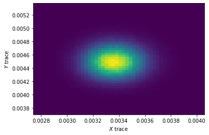
The expected output: 2d histogram shows correlation between X and Y because daily probabilities of success in example dataframe are correlated and model was supposed to catch this correlation.
What I got: 2d histogram shows no correlation.
The questions are:
-
Is the theoretical model correct and should it actually covariate X and Y?
-
If the answer is “yes” then how do I modify my PyMC3 model so it actually catches the correlation between conversion rates?