New sampling algorithm from a MCMC newbie

Hello !

Last weekend I watched this video about diffusion models and learned about Langevin diffusion.

(I am originally a C++ dev who is now doing a bit of python/pytorch)

This first seemed crazy to me that a random walk combined with a gradient descent on the log potential could get you this very potential (with the subtle sqrt(eps/2) mix) so I had to look into the proofs and I also had an idea about combining optimizer algorithm with Langevin diffusion.

The idea is pretty simple and after coding it up I found a paper from 2020 doing exactly what I did.

Then I learned about MALA, HMC and NUTS (this Hamiltonian idea is incredible) and I had an other idea for a sampler.

The issue with discretize langevin stepsize is you get some kind of convolution by a gaussian kernel of the posterior you are trying to sample. You can reduce the stepsize but you get much more autocorrelation.

My idea was to:

  • use many // chains using the modern vectorized hardware that we have
  • use adaptative gradients scheme as warmup since it would explore much faster
  • use subchains with a (1-t)^2 annealing schedule after warmup keeping only the last subchain sample

edit: the schedule idea is very similar to this paper I’m always 5/6 years late…

This way you progressively deacrease the variance of the noise kernel, get your sample and start again from large variance noise kernel. Since you go from enlarge fuzzy density to a much sharper image, it looks like a “vascularisation” of the distribution, hence the codename for this sampling algorithm: Hearbeat.

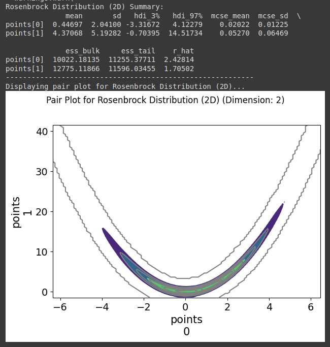
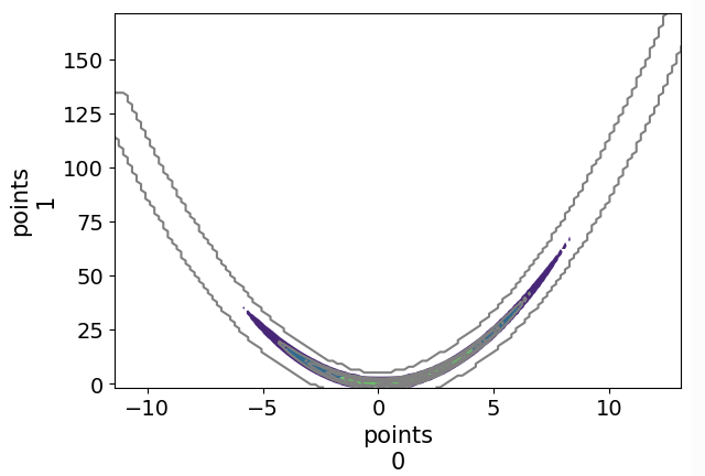
I wrote the sampler in pytorch and asked Gemini to recode it in JAX (got a x3 speed improvement) and I’ve tried running the sampler on a very simple mixture of gaussian against other JAX samplers from PyMC (numpyro and blackjax), and I get very comparable result for a very different algorithm. ^^ (note I used 1024 chains for my algo and 8 for the NUTS sampler to get similar running time, 8 chains seems to get the fastest ESS/sec for the NUTS samplers)

I ran on CPU without multithread and need to do much more tests with other distributions and on GPU. From what I get, it is much easier to tune my sampler to increase num_sample/ESS where for example the acceptance probability isn’t ideal for NUTS. It is also much much faster on CPU than NUTS sampler if you need many chains, I need to check this is also the case on GPU.

It is way too early to share but I’m too excited not to so here is a notebook if you want to play with it. I will see if I can provide a better support (colab?) later this we. Any comments are welcome. :slight_smile:

Colab link: Google Colab

Thank you for reading this far.

NB: Beware I am not a statistician and still very new to bayesian statistics.

4 Likes

Not sure why I cannot edit my post anymore but I ran it on 8 TPUv2 and get ~60k ESS/s with a ESS/num_samples > 0.99.

HeartBeat Summary:
              mean       sd   hdi_3%  hdi_97%  mcse_mean  mcse_sd  \
points[0]  1.20289  1.99133 -1.86957  5.21001    0.00138  0.00097   
points[1]  0.80211  1.72083 -2.38160  4.02596    0.00119  0.00080   

               ess_bulk      ess_tail    r_hat  
points[0]  2.082956e+06  2.091615e+06  1.00001  
points[1]  2.087530e+06  2.092678e+06  1.00003 

The x/y-variances and y-mean are within the 95% credible interval (if I am not mistaken) but the x-mean falls very close with a p-value of 4%. I am pretty sure there is bias from the annealing which you can alleviate with longer subchains/leaps (increasing num_steps) lowering ESS/sec but I think this kind of bias is acceptable in practice.

I should use some more complicated posterior than my 2D gaussian mixture in the future.

I did manage to make numpyro nuts sampler work on TPUs but it was so slow there must be something wrong (2min for 4 chains of 2048 samples) so I cannot do a comparison. Blackjax is the same. Will need to check on GPU (even discounting the initial model compilation).

1 Like

It seems to work well on Neal’s funnel (2D) and a mixture of 4 normalized 3D gaussians arranged in a circle of radius 5 around the origin (in the XY plane):


Neal's Funnel (2D) Summary:
              mean       sd   hdi_3%  hdi_97%  mcse_mean  mcse_sd  \
points[0]  0.00091  1.21372 -2.31871  2.36674    0.00200  0.00265   
points[1]  0.01961  1.73251 -3.24867  3.25367    0.00317  0.00450   

               ess_bulk      ess_tail    r_hat  
points[0]  399806.79379  409641.80882  1.00037  
points[1]  306966.41373  412366.67968  1.00075  


Multi-Modal Gaussian Mixture (3D, 4 modes) Summary:
              mean       sd   hdi_3%  hdi_97%  mcse_mean  mcse_sd  \
points[0] -0.00309  3.66542 -6.16030  6.19604    0.01239  0.00437   
points[1]  0.00650  3.68394 -6.17726  6.19660    0.01256  0.00435   
points[2]  0.00099  1.00450 -1.90596  1.87146    0.00098  0.00069   

               ess_bulk      ess_tail    r_hat  
points[0]  9.916165e+04  4.251901e+05  1.00955  
points[1]  9.735287e+04  4.176209e+05  1.01056  
points[2]  1.052703e+06  1.052718e+06  1.00000  

This is single threaded on Colab’s CPU. It took ~1min for the Funnel and ~3min on the gaussian mixture but I did very minimal finetunning.

I did implement an optimization for when the prior is bad and some chains diverge. After the adabelief stage I look at the norm of the gradient’s EMA, if it’s 0 I discard the chain and copy the state of an other non-diverging chain (but I did implemented it thinking some chains were diverging while it was in fact an issue in my implementation of the densities so it might not be needed).

The colab notebook is not yet updated with the latest code. I need to do some more tests, I’ll keep you updated. :slight_smile:

PS: I no longer have access to Colab’s free TPUs (might wait?) given how much faster it was I’m thinking about getting a Google cloud account…

PS2: The previous TPU run was done without parallelism which I think is not implicit with JAX so 7 out of 8 TPUs where idle.

1 Like

Another update, I’ve tried Neal’s funnel in 5D which converges easily but the evil log posterior is the Rosenbrock(a=1, b=100) with a temperature of 20.

I did not managed to make it converge:

I am pretty sure other MCMC sampler have the same issue with this posterior. The geometry of the ridge is too awful for the chain to get a good r_hat or ESS/num_samples.

Getting the “banana” density is easy though but you get why this is such a good function to test optimizers.

I will update the colab link tomorrow. Sorry for soliloquizing.

1 Like

Today’s update. I still did not change the Colab but I need to clean up the code.

I’ve helped Gemini (not the other way around ;)) parallelize the sampler onto multiple TPUs. Now I’m using all 8 TPUv2 so that’s ~1.5-2kW or 180 TFlops (F32) or a bit more than two 4090 GPUs.

Sampling for a bit more than 15min I get this for the exp(-Rosenbrock(a=1, b=100)/20):

Rosenbrock Distribution (2D) Summary:
               mean        sd   hdi_3%   hdi_97%  mcse_mean  mcse_sd  \
points[0]   1.01379   3.18565 -5.10063   6.98604    0.02000  0.01513   
points[1]  11.17613  15.88238 -0.82181  39.96727    0.11543  0.22649   

              ess_bulk     ess_tail    r_hat  
points[0]  25647.03811  19713.99465  1.03724  
points[1]  36724.02548  20675.96291  1.02565 

Note: the desmos graph I shared yesterday was for b=1 which is easy to sample from, you can set b to 100 with the slider but the graphing tool is glitching because of the shape of the function.

Still not perfect but I will stop there for now. Still should clean up the code and update the shared colab. :slight_smile:

1 Like

This is a pretty deep field, so I’d recommend doing some key background reading on Markov chains if you want to do MCMC. And then on some practical ways for evaluating them. If you’re OK with a bit of calculus, I’d highly recommend this overview from two of the leading experts in the field.

The intro chapter to the handbook of MCMC is good, as is Radford Neal’s chapter on HMC. They’re both free samples available on the book’s home page (just don’t take Geyer’s advice on how to evaluate real-world samplers—he’s a theoretician).

HMC can sample this. More diffusive samplers take a very long time. Because the posterior isn’t log concave and has varying curvature (alignment of the eigenvectors of the Hessian of the log density evaluated at a point in the posterior), it’s impossible to find a linear preconditioner like a mass matrix that transforms to standard normal. I’d highly recommend this paper of Agrawal and Domke’s on normalizing flows:

If you set a small enough step size, HMC is fine with this problem, as they show in the paper.

HMC is much better than Langevin at sampling precisely because it avoids the diffusive random-walk behavior of either random-walk Metropolis or Metropolis-adjusted Langevin. It’s why PyMC defaults to the NUTS sampler rather than to Langevin. In CS terms, diffusions (i.e., random walks) lead to \mathcal{O}(N) steps required for a new draw, in HMC it’s \mathcal{O}(N^{1/4})—this is the theoretical bound, but in practice, the constant terms are much better and in many cases, each iteration takes more than one effective draw.

There’s a big split in the field between adjusted and unadjusted methods. The latter typically go faster, but have some residual bias, which can be a win with few enough draws because the variance from the draws is larger scale than the bias early on. For example, people run Langevin without a Metropolis acceptance step—this is the go-to method for molecular dynamics simulation, for example.

2 Likes

Indeed HMC samples it just fine with good r_hat and ESS, I also found a huge bug with diverging chains in my sampler which seems to be causing a lot if issue I plan to fix it this evening (edit: still not fixed). I should have done more comparison with the pymc NUTS samplers.

Thank you for all the resources. I will try to read them.

PS: I thought normalizing flows were more used for variational bayes.

Edit: I suppose the Hamiltonian flow is normalizing because it preserve volume in phase space (with the nice property that the marginal distribution in positon is what we aim to sample from). I think I did not fully grasp the advantage of NUTS and HMCs. My algorithm is very hardware friendly hence it’s competitiveness for “reasonnable” densities sometimes beating NUTS by a lot but for more tricky distribution HMC allow you to take bigger steps. This was an interesting ride. I will try to iron out the bugs my jax implementation seems to have (like the Ess varies with the number of tpus used in // which is weird) and update this post once more.