Posterior predictive checks with Gaussian Process

Hi folks,

I can’t decide whether my model is wrong or I’ve misunderstood something. I’m using pymc v4 for a Gaussian Process (the marginal likelihood implementation - model explanation is at the end). My goal is to get estimates for the covariance hyperparameters.

Context
My posterior predictive check on the outcome is as follows:

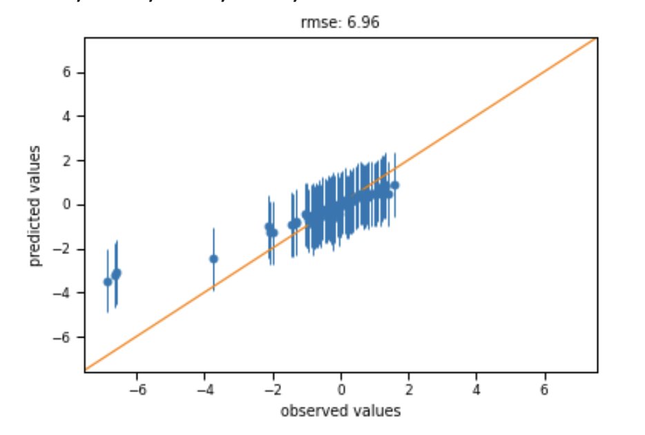
However, when I try and plot the mean predicted vs observed values I get a flat prediction:

I’ve tried fitting the GP using pm.find_MAP but this is highly dependent on the initial conditions (the start parameter) but it does give OK-ish predictions:

Question 1: is my calculation of the mean and standard deviation of p(\hat{y}_i|y_i) (y_mean/std above) correct? (FYI: I wouldn’t normally use the standard deviation - it’s just a quick and dirty way of getting errors for the purposes of this post.)

Question 2:

Asking for the other variables in the PPC function gives me drastically different values for the PPC of the outcome:

What is going on here? Shouldn’t PPC be independent of what variables you ask to draw from it?

Model explanation

with model: 
    gp = pm.gp.Marginal(cov_func=cov)
    y_ = gp.marginal_likelihood('y_', X=X, y=y, noise=sigma_n)
    trace = pm.sample(draws=1000, tune=1000, chains=2, cores=2, target_accept=0.90)

cov is a product of 5 exponential kernels over the columns of X and a general scale term:

eta = eta_prior('eta')
cov = eta**2
for i in range(X.shape[1]):
    var_lab = 'l_'+X_labels[i]
    cov = cov*pm.gp.cov.Exponential(X.shape[1], ls=l_prior(var_lab), active_dims=[i])

The priors are all weakly informative (prior predictive checks show that the outcome 90% of the time lies within the observed range). eta, sigma_n ~ HalfCauchy(1); all other parameters ~ Gamma(1, 0.5). The trace plots and summary statistics all show good convergence. Running it for 10’000 draws doesn’t materially change anything.

Thanks in advance!

ArviZ KDE doesn’t show anything outside the range of the data provided to it. The black line for the observed data indicates that there are no observations over ~2 even if there are a lot between 0-2. Is this a hard constraint on your data maybe? This behaviour is clearly not retrived by your model whose posterior predictive shows high probability for values over ~2. It also shows there are observations at ~7 behaviour again not present in your model whose posterior predictive gives virtually no probability there.

All your posterior predictive KDEs are centered around 0 as shown in the ppc plot and there is little to no asymmetry.

I think so but I never know what axis represent what :sweat_smile:. I always use named dims because I prefer them but also because I wouldn’t be able to do much otherwise. There is some wigglyness around 0 in the y axis which I think matches the means I’d make from the kdes in the ppc plot so I have no reason to suspect it is wrong.

You are generating prior predictive samples here. When sampling from the posterior predictive, pymc uses the values in the provided trace as default, then samples from the distributions with observed kwarg aka likelihood terms. However, if the name of a variable is given in var_names or it is missing from the provided trace, pymc will sample from its prior. This is needed in multilevel or random effect models for example to draw samples from the prior given the constraints the posterior sets on its parameters aka hyperpriors, but if you simple repeat all the variables in the model there you end up sampling from the prior and prior predictive distributions hence the way off range between -10k and 10k instead of -8 and 8.

1 Like

Wow - thanks very much for this response.

My outcome has been transformed to a scale which naturally stops at 2 (done for non-statistical reasons). Putting it back on the original scale doesn’t change anything though (predictions are still flat), except that the posterior and the range of observed values match up a bit better.

So your answer to question 1 is really all that I needed - I think my model is probably poorly specified.

I think some of the MAP estimates are locally optimized and give good predictions, but sampling over the full parameter space using NUTS washes them all out to give no predictive value.

I’m not sure I understand your answer to 2 though. The variables I named in the ppc function are actually in the model, so they should just come from the trace.

1 Like

If they are not in the trace or you pass include them in var_names they will be resampled (ignoring the value in the trace if any). If you only want posterior preditive samples for ppc checks just run sample_posterior_predictive without any arguments other than the trace. By using var_names you are modifying the default behaviour

Gotcha - thanks!