Posterior seems to capture right values but multiple posterior peaks suggest something is wrong

[mmn]

@pymc-bot
Hello everyone (bot included!).

I am working on a problem involving constructing and inverting a matrix formed by Legendre polynomials.

My problem is that I can see from the resulting posterior distributions, that the original values, which are generally quite close to zero, have been recovered in the peak of the distribution, however other modal peaks are observable. I would like to get rid of them.

I have experimented with Laplace and Normal distributions however the effect is the same. The run time is also quite long for this even with 1000 draws and 1000 tuning steps - suggesting to me that something inefficient is occurring.

The general thrust of the code is as follows

with pm.Model() as model:
    # # Use a function to describe varying gamma
    # Beta_pymc_1 = pm.Laplace("Beta_pymc_1", mu=0.1, b=0.001, shape=6)
    # Beta_pymc_2 = pm.Laplace("Beta_pymc_2", mu = 0.1, b = 0.00003, shape= 6 )  
    # Beta_pymc_3 = pm.Laplace("Beta_pymc_3",  mu =0.1, b = 0.00002 , shape= 6 )  
    # Beta_pymc_4 = pm.Laplace("Beta_pymc_4", mu = 0.1, b = 0.00005, shape= 6 )  
    
    Beta_pymc_1 = pm.Normal("Beta_pymc_1", mu=0.0, sigma=0.05, shape=6)
    Beta_pymc_2 = pm.Normal("Beta_pymc_2", mu=0.0, sigma=0.05, shape=6)
    Beta_pymc_3 = pm.Normal("Beta_pymc_3", mu=0.0, sigma=0.05, shape=6)
    Beta_pymc_4 = pm.Normal("Beta_pymc_4", mu=0.0, sigma=0.05, shape=6)
    
    
    # noise component
    sigma_noise = pm.HalfNormal("sigma_noise", sigma= 0.5)

    # Compute transformed gamma terms
    G11 = pt.dot(X_pt, Beta_pymc_1)
    G21 = -pt.dot(X_pt, Beta_pymc_2)
    G12 = -G21
    G33 = pt.dot(X_pt, Beta_pymc_3)
    G43 = pt.dot(X_pt, Beta_pymc_4)
    G34 = -G43

    # Efficient tensor construction of Gamma_model shape (n_freq, 4, 4)
    n_freq = G11.shape[0]
    zero = pt.zeros_like(G11)

    row0 = pt.stack([G11, G21, zero, -G43], axis=1)
    row1 = pt.stack([G12, G11, zero, zero], axis=1)
    row2 = pt.stack([zero, zero, G33, G34], axis=1)
    row3 = pt.stack([G43, zero, -G34, G33], axis=1)

    Gamma_model = pt.stack([row0, row1, row2, row3], axis=1)  # shape (n_freq, 4, 4)
    Gamma_model = pm.Deterministic("Gamma_model", Gamma_model)

     #Next steps perform the inverse operation
     # 1: obtain INV_BRACKET = pt.linalg.inv(A+ Gamma_model)

    # 2: Use INV_BRACKKET within a larger matrix expression to get Y

    likelihood = pm.Normal("likelihood", mu=Y, sigma = sigma_noise, observed=data)

an example of one set of Beta values to infer

0.0135227
0.00814225
0.0092286
0.00346928
-0.0111075
-0.000543785

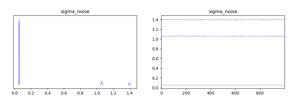
and the post inference results.

zoomed in to the key region

If there is anyone out there who can help with this I would be most grateful.

[bob-carpenter]

I would guess it’s noise coming from the kernel density plot. The reason I say that is that samples are less concentrated by construction in the tails. If your kernel density estimator has a narrow bandwidth, this is what things look like. Try just generating some randomly distributed data and plotting it with your density estimator to see what it looks like. Especially if you can plot something with slightly longer tails than normal.

If your R-hat convergence diagnostics and effective sample sizes are good, you should be fine.

If you’re really worried about it, do posterior predictive checks on quantities of interest. That’s always good practice anyway because it will also test if your model’s well enough specified predictively for your quantities of interest.

Rescaling the Beta_pymc_1 or providing well-scaled initializationm may also help speed up computation given the narrow priors. Also, standardizing the preidctors may also help with scale.

You might be able to speed up some of the computations by using linear algebra rather than all t his matrix manipulation, which applies a lot of memory pressure, which is often a bottleneck, especially when running multiple chains in parallel.

[jessegrabowski]

What code did you use to sample the model?

[mmn]

Hi @jessegrabowski, something like the following if that’s what you mean..?

with model:
    trace = pm.sample(
       draw = 2000,
        tune= 2000,
        chains=4, 
        target_accept=0.95,
        return_inferencedata=True,
        discard_tuned_samples=False)

@bob-carpenter thanks for the response - something for me to check out and, as suggested, I have been playing with priors and posterior checks. Some of my convergence stats are poor, as well as this effect occurring, leading me to think it was not a KDE error.

I was able to slightly improve things with less informed priors

    Beta_pymc_1 = pm.Normal("Beta_pymc_1", mu=0.0, sigma=1, shape=6)
    Beta_pymc_2 = pm.Normal("Beta_pymc_2", mu=0.0, sigma=1, shape=6)
    Beta_pymc_3 = pm.Normal("Beta_pymc_3", mu=0.0, sigma=1, shape=6)
    Beta_pymc_4 = pm.Normal("Beta_pymc_4", mu=0.0, sigma=1, shape=6)
        
    # noise component
    sigma_noise = pm.HalfNormal("sigma_noise", sigma= 1)

resulting in the below posteriors for beta_1

the noise posterior tells a similar tale

and I can see that some of the chains are not mixing - which probably puts the KDE noise aspect to bed? True values for sigma_noise = 0.05 and Beta_pymc_1 = 0.00338067.

and finally, from the posterior predictive check - I note that the peak of the PPC mean is way off the true peak.I suppose this why simga noise was often inflated to compensate. I am struggling to see which further tweaks might benefit. Frustrating since the posteriors show that a modal peak is “in there”.

Inference summary stats below if useful.

[jessegrabowski]

Some thoughts:

1. If you look at the likelihood of samples from each chain, are they roughly equal (that is, are the solutions found by each chain equi-probable explanations for the data, or are some bad initializations just getting stuck?)
2. On that subject, you might have to be more sensitive about the initialization, using draws from the prior for example, instead of uniform jitter on arbitrary initial points (this is the default).
3. Do you have any scientific intuition about these parameters that you can use to pin down the solution space more aggressively? For example, is beta_1 = 0.12 reasonable? What about beta_1 < 0?
4. You’re cranking up target_accept – presumably to avoid divergences? But if you have to do this your posterior geometry is likely difficult. Your model might be a good candidate for normalizing flow sampling in nutpie – I’ve had success using this on models with a lot of hairy linear algebra

[bob-carpenter]

@mmn

Some of my convergence stats are poor

That would certainly cause bumps in the KDE plots. If you haven’t gotten reasonable convergence diagnostics, that’s always the place to start fixing.

[mmn]

@jessegrabowski

On that subject, you might have to be more sensitive about the initialization, using draws from the prior for example, instead of uniform jitter on arbitrary initial points (this is the default).

Hi @jessegrabowski

Thank you so much for those thoughts. It seemed to me on reflection that some chains were stuck. Indeed, at the first go, setting consistent intivals and removing the jitter did the trick

initvals = {
    "Beta_pymc_1": np.zeros(6),
    "Beta_pymc_2": np.zeros(6),
    "Beta_pymc_3": np.zeros(6),
    "Beta_pymc_4": np.zeros(6),
    "sigma_noise": 0.05
}

with model:
    trace = pm.sample(
       draw = 1000,
        tune= 1000,
        chains=4, 
        init="adapt_diag",
        initvals = initvals,
        return_inferencedata=True,
        discard_tuned_samples=False)

This resulted in some lovely-looking distributions. The below is for 1000 runs which I am very pleased with. Other beta coefficients looked similarly good.

The value for sigma noise is off - however it is a small value to start with so I am not so concerned with this. One to tweak perhaps. I will look into your other thoughts too.

@bob-carpenter, happy to report that these fixes result in a stronger posterior PPC (zoom in section below) along with some healthy convergence stats (last figure below).

Thank you both so much for your input. Looking forward to a good night’s sleep now! Happy to receive pointers if my tweak was less than ideal but will mark this as a solution for now.