I’m using gp.Latent as a (top-level) prior in a hierarchical GLM to estimate parameter values in a mechanistic model of timeseries data (experimental instrument readings). The parameter estimates are well-defined and reasonable, but when I go to predict new parameters using gp.conditional the GP draws don’t appear conditioned on the estimates. Even supplying the posterior estimates as given I just get flat predictions with broad, uniform variance. However, if I then use gp.Marginal to regress a GP on the posteriors using the same priors on the hyperparameters, the GP draws fit the data nicely. I’ve put a “toy” example in this colab notebook. (Sorry, it takes ~30-60 minutes to run on colab, it was the simplest I could make it while retaining the structure.)
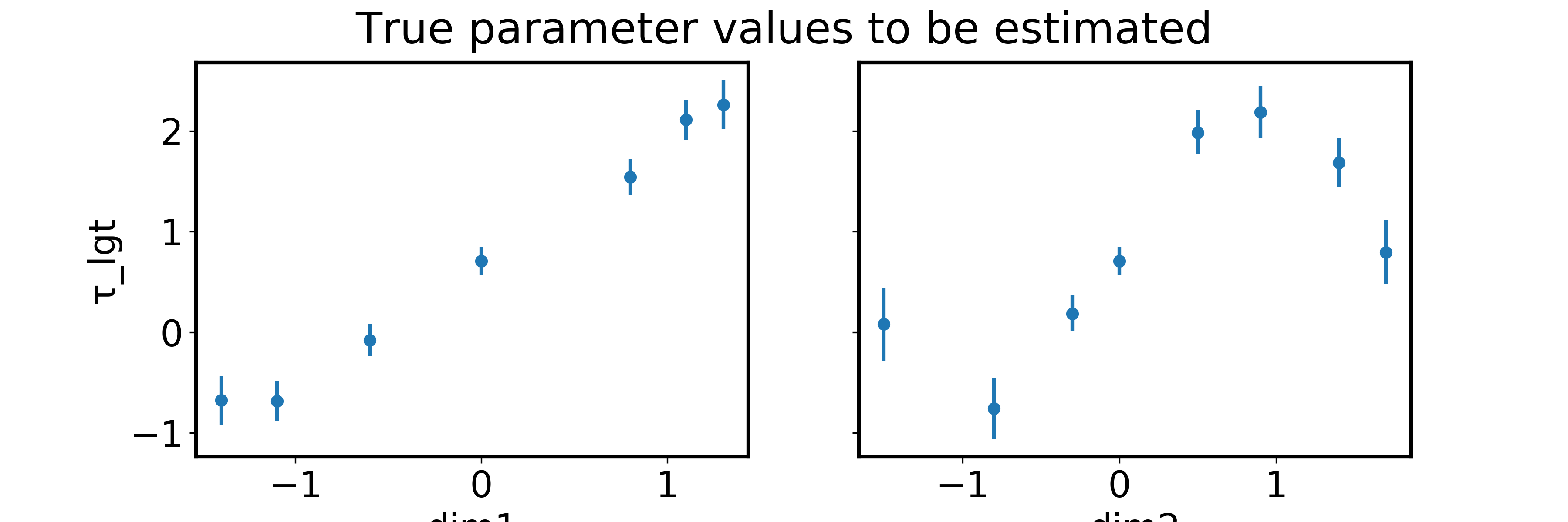
The “true” parameter values (as estimated without the GP) are very close to the fake ones I generate in the notebook. (Note, despited the appearance of dim2, I don’t want to use a periodic kernel; I don’t expect to observe much beyond the extents of this plot.)
Fake experimental measurements, ~50 timepoints each:

The model looks like this. I have 14 groups (reaction conditions), each of which has 2 replicates. Each group is assumed to have a typical parameter value from which individual reactions can vary slightly. The groups are defined by two components, called dim1 and dim2 below. The parameter τ (under an appropriate transform) varies very close to linearly along dim1, but has more complex behavior along dim2, hence the GP. My actual model has four parameters, each estimated with a similar hierarchical GLM structure, albeit without a GP component (for now).
S_obs = np.hstack(data.sig)
grp = data.group.values
n_grps = len(set(grp))
n_pts = data.sig.map(len)
rxn = np.hstack([int(i)*np.ones(n, dtype=int) for i,n in enumerate(n_pts)])
n_rxns = len(set(rxn))
t = np.hstack(data.time)

dim2_lst = np.sort(list(set(dim2)))[:,None]
dim2_idx = [list(dim2_lst).index(v) for v in dim2]
dim2_new = np.linspace(dim2_lst.min()-0.25,dim2_lst.max()+0.25,100)[:,None]
coord1 = theano.shared(dim1)
coord2 = theano.shared(dim2)

with pm.Model() as latent_model:
    # Dim1 behaves nearly linearly
    τ_lgt_β_dim1 = pm.Normal('τ_lgt_β_dim1', mu=0, sigma=0.5)

    # Dim2 behavior is more complicated, requiring a GP
    ℓ = pm.InverseGamma('ℓ', mu=1.7, sigma=0.5)
    η = pm.Gamma('η', alpha=2, beta=1)
    cov = η**2 * pm.gp.cov.ExpQuad(1, ℓ)
    gp = pm.gp.Latent(cov_func=cov)
    τ_lgt_β_dim2 = gp.prior('τ_lgt_β_dim2', X=dim2_lst)

    ## Group-level hyperpriors
    # Expected value of τ based on dim1 and dim2
    τ_lgt_μ_grp = pm.Deterministic('τ_lgt_μ_grp', τ_lgt_β_dim1*coord1 + τ_lgt_β_dim2[dim2_idx])
    # Non-centered parameterization of actual value of τ for each group
    τ_lgt_μ_grp_σ = pm.Exponential('τ_lgt_μ_grp_σ', lam=1)
    τ_lgt_μ_grp_nc = pm.Normal('τ_lgt_μ_grp_nc', mu=0, sigma=1, shape=n_grps)
    τ_lgt_μ = pm.Deterministic('τ_lgt_μ', τ_lgt_μ_grp_nc*τ_lgt_μ_grp_σ+τ_lgt_μ_grp)

    # Non-centered parameterization of actual value of τ for each reaction
    τ_lgt_σ = pm.Exponential('τ_lgt_σ', lam=1)
    τ_lgt_z_nc = pm.Normal('τ_lgt_z_nc', mu=0, sigma=1, shape=n_rxns)
    τ_lgt_z = pm.Deterministic('τ_lgt_z', τ_lgt_z_nc*τ_lgt_σ+τ_lgt_μ[grp])
    # Un-transform τ back to the natural scale
    τ_lgt = pm.Deterministic('τ_lgt', τ_lgt_z*scale+shift)
    τ = pm.Deterministic('τ', pm.invlogit(τ_lgt))

    σ = pm.Exponential('σ', lam=1)

    # Simplified mechanistic model
    S = 1 / (1+pm.math.exp(t/τ[rxn]))
    S_lik = pm.StudentT('S_lik', nu=3, mu=S, sigma=σ*np.exp(-7), observed=S_obs)
After running pm.sample(), I draw predictions from the Latent GP:
with latent_model:
    τ_new = gp.conditional('τ_new', Xnew=dim2_new, given={'X':dim2_lst,
                                                      'y':trace['τ_lgt_β_dim2'].mean(axis=0)[:,None],
                                                      'noise':trace['τ_lgt_β_dim2'].std(axis=0)[:,None],
                                                      'gp':gp})

    gp_draws = pm.sample_posterior_predictive([trace], vars=[τ_new], samples=1000)
The parameter estimates are very close to their true values. The estimates of τ_lgt_β_dim2 along this axis are shown as white circles below, with the respective τ_lgt_μ values as blue circles. However, gp.conditional is giving what appears to be a GP conditioned on nothing at all.

On the other hand, if I directly regress on the posterior estimates of τ_lgt_β_dim2, the result is as expected:
with pm.Model() as marginal_model:
    ℓ = pm.InverseGamma('ℓ', mu=1.7, sigma=0.5)
    η = pm.Gamma('η', alpha=2, beta=1)

    cov = η**2 * pm.gp.cov.ExpQuad(1, ℓ)
    gp = pm.gp.Marginal(cov_func=cov)

    grp_τ = gp.marginal_likelihood('grp_τ', X=x, y=y, noise=e)

    mp = pm.find_MAP()
    trace_marginal = pm.sample()

with marginal_model:
    τ_new = gp.conditional('τ_new', dim2_new)

    map_samples = pm.sample_posterior_predictive([mp], vars=[τ_new], samples=1000)
    full_samples = pm.sample_posterior_predictive([trace_marginal], vars=[τ_new], samples=1000)

...

My main question is, how do I get better predictions from the latent GP? Is this difference between Latent and Marginal implementations expected, or have I made a mistake?
As a side note, please let me know if you have suggestions for analyzing this sort of timeseries data with a mechanistic model better. The point-by-point likelihood evaluation seems inefficient (my real dataset ~11000 points, and I expect it to grow by two or three fold) and naive, ignorant of the inherent correlation in points (and therefore likelihoods) resulting from a given set of parameters.


