Saturating growth model for binomial data

I need to estimate a probability from a set of successes observed over time. I this application I have multiple ‘looks’ at the data, and need to estimate ‘p’ from this.

Because of this, i thought that a simple Binomial model with saturating growth would be a good place to start:

import pandas as pd
import numpy as np
import pymc3 as pm
import matplotlib.pyplot as plt
import seaborn as sns
import theano.tensor as tt

%matplotlib inline
plt.rcParams.update({'font.size': 20})
%config InlineBackend.figure_format = 'retina'
SEED = 48

def logistic(K, r, t, C_0):
    A = (K-C_0)/C_0
    return K / (1 + A * np.exp(-r * t))

data = {
    'y': [1, 20, 30, 55, 80, 95, 105, 110, 111, 112],
    'n': [1000, 1000, 1000, 1000, 1000, 1000, 1000, 1000, 1000, 1000]
}

t = np.linspace(1, 10, 10)

with pm.Model() as binomial_model:

    C_0 = pm.Normal("C_0", mu=0.001, sigma=10.0)
    r = pm.Normal("r", mu=0.02, sigma=0.5)
    K = pm.Normal("K", mu=0.0, sigma=1.0)

    # saturating growth
    growth = logistic(K, r, t, C_0)

    p = pm.Deterministic("p_t", pm.invlogit(growth))    
    # likelihood
    pm.Binomial('y', n=data['n'], p=p, observed=data['y'])

pm.model_to_graphviz(binomial_model)

with binomial_model:
    train_trace = pm.sample(1000, tune=1000, chains=4, return_inferencedata=True)
    pm.traceplot(train_trace)
    pm.plot_posterior(train_trace)
    ppc = pm.sample_posterior_predictive(train_trace)

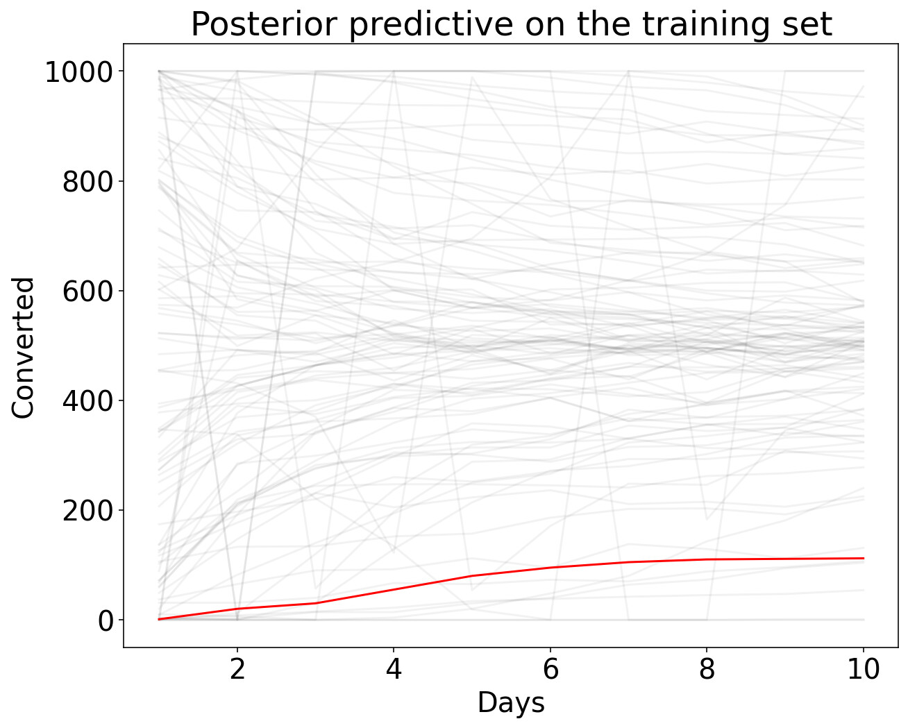
And this model is being fit, and producing reasonable posterior predictions.

fig, ax = plt.subplots(figsize=(10, 8))
ax.plot(t, ppc['y'].T, ".k", alpha=0.05)
ax.plot(t, data['y'], color="r")
ax.set(xlabel="Days", ylabel="Converted", title=f"Posterior predictive on the training set")

But I’m a bit concerned that it’s producing multi-modal posteriors (even if one mode contains the truth).

What steps could I take to prevent this, and use better priors?

Hi @TomKealy
My recommendation would be to explore more constrained priors so that prior predictive checks give rise to what you consider to be meaningful outputs.

# prior predictive checks

with binomial_model:
    prior_checks = pm.sample_prior_predictive(samples=100)
    
fig, ax = plt.subplots(figsize=(10, 8))
ax.plot(t, prior_checks['y'].T, "k", alpha=0.05)
ax.plot(t, data['y'], color="r")
ax.set(xlabel="Days", ylabel="Converted", title=f"Posterior predictive on the training set")

gives

So we can see that the combination of the model + priors is giving rise to all kinds of predictions. Some of these might seem 'reasonable, but some might not. So I’d recommend first just exploring what ranges of parameters give rise to sensible predictions in the first place, then constraining your priors based on that.

It might also be that the model itself is a bit iffy - keep an eye on the sampling and divergences. Maybe refining priors will fix that, maybe the model needs to be looked at. Maybe there’s a way to make the model simpler?

1 Like

Hi @drbenvincent, was just replicating this in pymc v4. To plot prior checks with an inference data object, is this the standard procedure?

ax.plot(t, prior_checks.prior_predictive['y'].stack().transpose()[:,:,0], "k", alpha=0.05)

It generates the same output as above, but wasn’t sure if there was a more straightforward way

Hi

prior_checks.prior_predictive['y'].squeeze().transpose()

It is definitely worth spending a bit of time learning about xarray. At the start I was a bit reluctant, but it can be handy, especially when you start to have more complex models and use named dimensions

2 Likes

Awesome. Thanks so much!