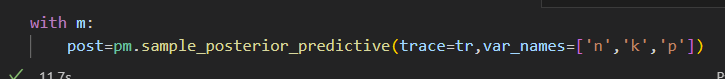
i am trying to create a simple model of a coin toss experiment:
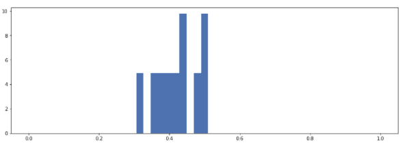
I want to use uninformed priors to see if i can capture the behavior after a sufficient amount of experiments. But I always end up with with something similar to the following for p and n posterior:
The model is capturing the true values of the process, so it seems like there is something right with the model rather than wrong!
If I understand correctly, you want do update the prior step by step, with one piece of data at a time, and plot how the posterior evolves as the data comes in? Since it’s just a simple binomial process, you could start with a Beta(0.5, 0.5) distribution (uniform over 0,1) and use the fact that beta and binomial are conjugate to get closed form solutions for the updates. The Wikipedia article on conjugate priors spells out how to do it for exactly this example.
But you don’t estimate N in this setting, because you are sitting there watching the coin flip and trying to judge the probability of heads, so you know N. In your setting, you have some one batch of fixed data and you don’t know N or p, so there’s no iterative process to go through to get from the prior to the posterior.
I am not necessarily interested in seeing the update point by point but rather the final posterior after Y experiments.
“you have some one batch of fixed data and you don’t know N or p, so there’s no iterative process to go through to get from the prior to the posterior.”
This is correctly interpreted how I want to setup the experiment and the model, with 2 free variables n and p. I thought that n , p → N, P as n_experiments would get bigger. But what I see is not that behavior and I am somewhat surprised about the large uncertainty.
The plots in the first post were at n_experiments=100, while the second are at n_experiments=1000? Between them, the variance in the posterior of both P and N has shrunk considerably, and the mean of the posterior distribution is zeroing in on the true parameter value. I don’t think you’re doing anything wrong.
Hi!
I agree that in the above results, the posterior of both P and N seem to zero in on the true parameter value, but in my experience that is not always the case for this model.
I took the time to rerun @maab’s example, with n_experiments = 10000.
In this ecample, there posteriors have zeroed in on the wrong values (see code and plot below). Each sampling chain also zeros in on different values with confidence (small posterior std).
I am questioning if one can actually estimate both N and P with confidence when the observed values are number of heads?
N=12
P = 0.5
n_experiments=10000
obs=np.random.binomial(N,P,n_experiments) #  observed number of heads with random number of flips

with pm.Model() as m:
    n = pm.DiscreteUniform('n', 1, 50)                  # unknown number of coin flips
    p = pm.Uniform('p', 0., 1., transform=None)         # P(A) probability of head before evidence (prior)
    y = pm.Binomial('k', n, p, observed=[obs])       # outcome of total model
    trace = pm.sample(10000,tune=1000,step=pm.Metropolis())
    pm.traceplot(trace)
I was currently evaluating the results at n_experiments = 1000 and given jessegrabowski’s answer above I felt confident that everything was working as planned. I think that I previously had to high expectations on how fast p and n should zero in on the true values.
However, following BjornHartmann’s suggestion to continue increasing n_experiments to 10000, I also get some weird results. Here is the traceplot (I ran this with chains=10):
It seems that each chain is homing in on a different solution giving weird results. Here are the overall plots of p,n:
p
n
So it seems that somewhere in the interval n_experiments=1000 - 10000, the model starts to deviate from the true values.
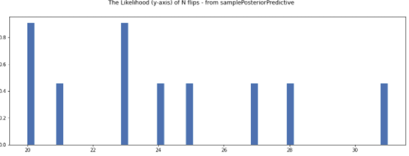
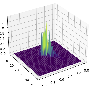
Following @junpenglao presentations on likelihood functions i have plotted the following likelihood function using the trace of p and n
Am i somehow “messing” up the likelihood function because of the large number of observed and getting the gradient to large ?
I am feeling rather confused at the moment, anyone has an explanation for this ?
Having looked at it a bit closer, I see now that your problem is under-identified. You are trying to estimate two parameters from only one data point, which means there is an infinite combination of solutions.
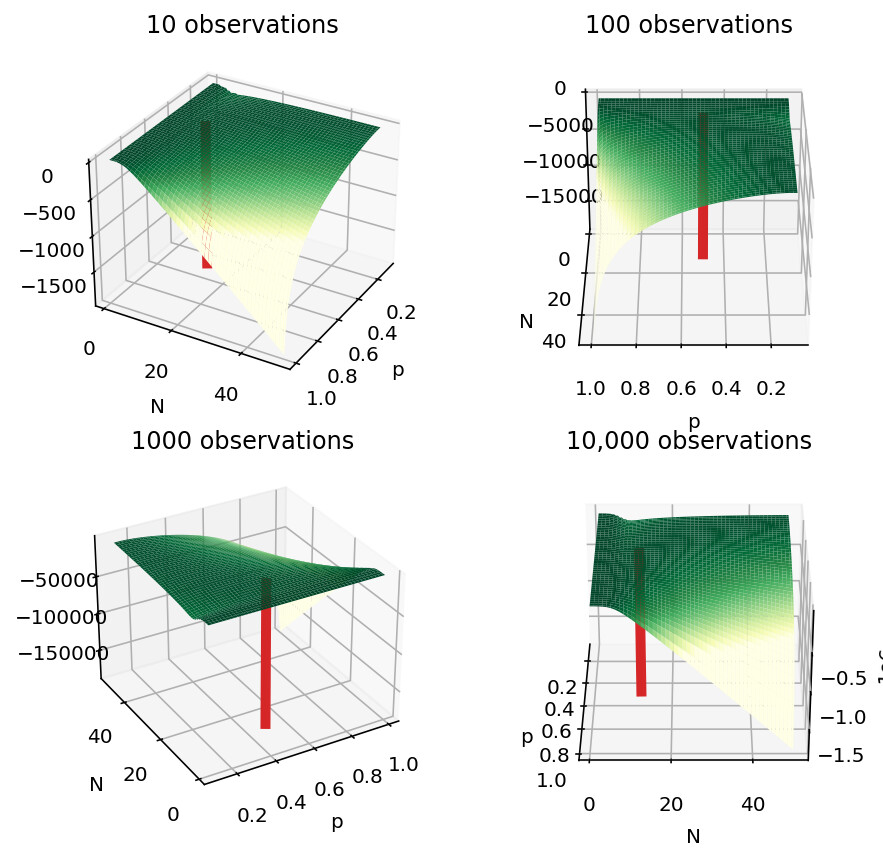
Since there are only two parameters, we can visualize the log likelihood function. I plotted it using a 100x100 evenly spaced grid for p and N, for 10, 100, 1000, and 10,000 observations. Note that the shape of the likelihood function is not a function of the number of observations, only the magnitude increases since it’s summing over more stuff. The shape is the same in all the pictures I just rotated it so we an get a better view. The true parameter values are at the red column. The little bump up when N is small is because I set all likelihoods where obs > N to 0; that doesn’t really exist.
You can see that the gradients of the function are essentially zero once you get up the hill that falls down towards N=50 and P=1. In particular, the true values are sitting squarely in the middle of the plateau. From the perspective of the sampler, all the points at the top of the plateau are going to be equally good.
The results @BjornHartmann got are due to how samplers explore a posterior space. Once a chain wandered somewhere onto the plateau, it will be very difficult to accept a move, so it just stays put (Metropolis specifically uses draws from a normal to randomly accept moves to parameters with equal or lower log probability, so curves you see in the trace are likely equal to this acceptance probability). If you actually evaluate the log probability of some data at p=0.24, n=19 and p=0.32 n=25, they are roughly equal, so the sampler is giving you two possible solutions (out of infinity).
I’m sure if you colored the chains in @maab 's trace plot (so we can tell which N goes to which p) and computed the log probs, you would find that all 10 are equivalent solutions.
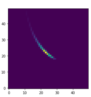
Another way to see this degeneracy is to look at the pair plots from the trace:
As you can see, the parameters are just a deterministic function of each other.
This is just the points that were sampled. You can even see the burn-in, where the sampler made it’s way up onto the plateau, then wandered around in a circle. See how it “spawned” on the hill part, at large N, so it had a gradient to climb over there.
To see the entire log-likelihood surface, I just made a grid of N and p, then evaluated the log-likelihood at each point using scipy. Something like:
N_grid = np.arange(1, 50)
p_grid = np.linspace(0.01, 0.99, 100)
results = np.zeros((50, 100))
for i, n in enumerate(N_grid):
    for j, p in enumerate(p_grid):
        d = scipy.stats.binom(p=p, n=n)
        logprobs = d.logpmf(obs)
        results[i, j] = lobprobs[np.where(logprobs != -np.inf)].sum()
A thousand thanks for that @jessegrabowski , it helped understand a bit more.
Although I still have even more questions
By actually plotting the log-likelihood i get the same shape as you posted above. I had already done it in non log space and I see a world of difference in the two.
Here is contour plot of the likelihood (sorry about the scale on x axis (p)) (a)
and here is the corresponding log-likelihood (b):
So, by looking at (a) it seems that the likelihood has a local maximum at approx. the true values of p,n. And indeed the model seems to home in on that when n_experiments is somewhere ~ 1000.
Looking at (b) i now agree with what @jessegrabowski posted above, but how can we explain 1) in this context, is it just random that the true values seem to be found in this case ? (I have not yet really experimented with changing N=20 and P=0.5 as shown in the first post)