Zero-inflated Student-T

Hi All,

I implemented a zero-inflated student-t distribution. Would you mind taking a look to see if it’s correct? Particularly I find the extreme values that are in both my prior- and posterior predictive checks a bit curious. I guess a student-t would allow for such values to pop up?

I would also like to know if my logp is correct. In the zero-inflated beta distributions I found here and here, when value = 0, only tt.log(self.pi) is returned. I do not understand why. Shouldn’t we also add pi * p(x=0|params) to this, like in ZeroInflatedPoisson for example?

Btw in my implementation, pi = probability of zero, so opposite to ZeroInflatedPoisson and the like.

class ZeroInflatedStudentT(pm.Continuous):
    def __init__(self, nu, mu, sigma, pi, *args, **kwargs):
        super(ZeroInflatedStudentT, self).__init__(*args, **kwargs)
        self.nu = tt.as_tensor_variable(pm.floatX(nu))
        self.mu = tt.as_tensor_variable(mu)
        lam, sigma = pm.distributions.continuous.get_tau_sigma(tau=None, sigma=sigma)
        self.lam = lam = tt.as_tensor_variable(lam)
        self.sigma = sigma = tt.as_tensor_variable(sigma)
        self.pi = pi = tt.as_tensor_variable(pm.floatX(pi))
        self.studentT = pm.StudentT.dist(nu, mu, lam=lam)
        
    def random(self, point=None, size=None):
        nu, mu, lam, pi = pm.distributions.draw_values(
            [self.nu, self.mu, self.lam, self.pi], 
            point=point, size=size)
        g = pm.distributions.generate_samples(
            sp.stats.t.rvs, nu, loc=mu, scale=lam**-0.5, 
            dist_shape=self.shape, size=size)
        return g * (np.random.random(g.shape) < (1 - pi))
    
    def logp(self, value):
        logp_val = tt.switch(
            tt.neq(value, 0),
            tt.log1p(-self.pi) + self.studentT.logp(value),
#             tt.log(self.pi))
            pm.logaddexp(tt.log(self.pi), tt.log1p(-self.pi) + self.studentT.logp(0)))
        return logp_val 

Generate fake data:

prob_dropout = 0.3
mean_expr = 5
n = 300
dropouts = np.random.binomial(1, prob_dropout, size=n)
expr = (1 - dropouts) * sp.stats.t.rvs(df=2, loc=mean_expr, scale=3, size=n)
plt.hist(expr, bins=50);

image

Prior predictive

with pm.Model() as t_model:
    p = pm.Normal('p', 0, 1.5)
    pi = pm.Deterministic('pi', pm.math.invlogit(p))
    mu = pm.Normal('mu', 0, 10)
    sigma = pm.Exponential('sigma', .5)
    nu = pm.Gamma('nu', alpha=5, beta=2)
    obs = ZeroInflatedStudentT('obs', nu=nu, mu=mu, sigma=sigma, 
                               pi=pi, observed=expr)

    priorpred = pm.sample_prior_predictive()
fig, axs = plt.subplots(figsize=(12, 3), ncols=5)
axs[0].hist(priorpred['pi'], bins=20); axs[0].set_title('pi')
axs[1].hist(priorpred['mu'], bins=20); axs[1].set_title('mu')
axs[2].hist(priorpred['sigma'], bins=20); axs[2].set_title('sigma')
axs[3].hist(priorpred['nu'], bins=20); axs[3].set_title('nu')
axs[4].hist(priorpred['obs']); axs[4].set_title('obs') #, bins=50); 
fig.tight_layout()

Sample.

with t_model:
    trace = pm.sample()
pm.traceplot(trace);

Posterior predictive.

with t_model:
    postpred = pm.sample_posterior_predictive(trace, var_names=['obs'])
    t_idata = az.from_pymc3(trace, posterior_predictive=postpred, prior=priorpred)
az.plot_ppc(t_idata);

image

plt.hist(postpred['obs'].flatten(), bins=2000, alpha=.3, label='Predictive');
# Limit x-axis so we can actually see the distribution
plt.xlim(-30, 30)

image

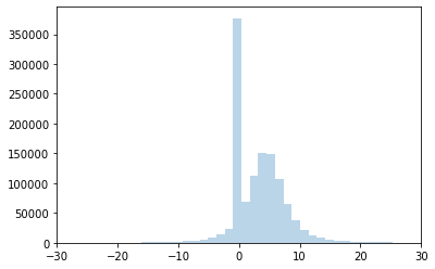
plt.hist(expr, bins=30, alpha=.3, label='Data');

image

Thanks!!

Hi, your code looks correct to me. In fact, I used your code and tested it on a dataset and it works quite fine.

Regarding your question, I agree with you, I think that the code in the linked post lacks the likelihood of the Gamma (not beta, right?) distribution for the x=0 branch.

1 Like

Hi,
a follow-up post: I was playing with this model and found that I had some problems in fitting it. After a while, that I was doing something stupid: Naturally, I wanted to standardize the data to make the definition of priors easier. So, what I was doing was: I transformed the non-zero values, assumed to be Gaussian or StudentT distributed, to mean 0 and std 1, leaving the zero values (the inflated values) at zero.

That brought me into trouble because now all of a sudden it is much hard to distinguish the normally (or studentT) distributed values from the inflated zero values. So, to remedy this, I would implement a more general InflatedStudenT (or InflatedGaussian) that takes an additional parameter, say N_inflation, which indicates the value that is being inflated.

Thus, to benefit from both the standardization of the non-zero values and keep the original relation between non-zero and zero values intact, one can transform all values by standardizing them and then use the new values of the zero values as N_inflation.

  • standardize the data
from sklearn.preprocessing import StandardScaler
scaler = StandardScaler()
ind = X != 0
scaler.fit(X[ind, None])
X = scaler.transform(X[:, None])[:, 0]
N_inflation = - scaler.mean_ / scaler.scale_
  • Fit the model with e.g. InflatedStudentT(nu, mu, sigma, pi, N_inflation=100)
with pm.Model() as model:
    mu = pm.Normal('mu', 0., 1.)
    sigma = pm.Exponential('sigma', 1.)
    p = pm.Beta('p', alpha=1., beta=1.)
    InflatedStudentT('obs', nu=2, mu=mu, sigma=sigma, psi=p, N_inflation=N_inflation,
                   observed=X)
    
    trace = pm.sample(1000, tune=2000)
  • For prediction, apply the inverse transformation from above.

Does that make sense?

I don’t quite see why a zero student t is useful (or any discrete and continuous mixture). By the fact that the Tstudent is continuous any value that is exactly zero ought to belong to the zero mixture with almost probability of 1 (and vice versa for any other value). Am I missing something?

On a second hand: I see the appeal of just passing in the raw data. My thinking is that for the purpose of inference one could as easily model the proportion of zeros with a Binomial distribution and use the nonzero values to model the tStudent distribution.

1 Like

And that’s why the logp of the gamma at zero was not in the original linked example. It’s wrong to compare a density and probability in equal terms.

That example was correct in assigning all the zeroes to the zero mixture and all the nonzeroes to the gamma component.

This would be the correct logp:

def logp(self, value):
        logp_val = tt.switch(
            tt.neq(value, 0),
            tt.log1p(-self.pi) + self.studentT.logp(value),   
            tt.log(self.pi))
            # pm.logaddexp(tt.log(self.pi), tt.log1p(-self.pi) + self.studentT.logp(0)))
        return logp_val

Thank you @ricardoV94 , what you’re saying makes sense to me.