Bayesian HoltWinters Implementation

Hello, guys.

I trying to learning PYMC by reimplementing some classical time series models. Now I’m stuck with is the most simple HoltWinters Exponential Smoothing model. It is just an additive and additive damped. In the frequestist implementation we just minimize the SSR of the following function:

def holt_add_dam(double[::1] x, HoltWintersArgs hw_args):
    """
    Additive and Additive Damped
    Minimization Function
    (A,) & (Ad,)
    """
    cdef double alpha, beta, phi, betac, alphac
    cdef double[::1] err, l, b
    cdef const double[::1] y
    cdef Py_ssize_t i

    err = np.empty(hw_args._n)
    alpha, beta, phi, alphac, betac = holt_init(x, hw_args)

    y = hw_args._y
    l = hw_args._l
    b = hw_args._b
    err[0] = y[0] - (l[0] + phi * b[0])
    for i in range(1, hw_args._n):
        l[i] = (alpha * y[i - 1]) + (alphac * (l[i - 1] + phi * b[i - 1]))
        b[i] = (beta * (l[i] - l[i - 1])) + (betac * phi * b[i - 1])
        err[i] = y[i] - (l[i] + phi * b[i])
    return np.asarray(err)

To start I tried to implement the following code.

def step(*args):
    y_tm1, l_tm1, b_tm1, α, β, ϕ = args
    
    l = alpha * y_tm1 + (1 - alpha) * (l_tm1 + phi * b_tm1) # update the level
    b = beta * (l - l_tm1) + (1 - beta) * phi * b_tm1 # update the trend

    μ = l + ϕ * b # forecast
    
    return (l, b, μ), collect_default_updates(inputs=args, outputs=[μ]) 
    
with pm.Model() as model:
    alpha = pm.Uniform('alpha', 0, 1)
    beta = pm.Uniform('beta', 0, 1)
    phi = pm.Uniform('phi', 0.8, 0.98)
    sigma = pm.HalfNormal('sigma', 0.1) # variance
    
    l0 = pm.Normal('l0', Y[0], 0.1) # initial level
    b0 = pm.Normal('b0', 0, 0.1) # initial trend
    yend = pm.Normal('yend', Y[-1], 0.1) # end value
    
    # Observed Data
    y_obs =  pm.MutableData('y_obs', Y)
    
    [l, b, yhat], updates = scan(fn=step,
                                    sequences=[{'input':y_obs, 'taps':[0]}],
                                    outputs_info=[l0, b0, None],
                                    non_sequences=[alpha, beta, phi],
                                    strict=True)
    
    pm.Normal('obs', mu=yhat, sigma=sigma, observed=y_obs)

This takes hour and hours to sample what is some how impossible as the frequestist approach takes seconds or few minutes by gridsearching. So, then I tried to change a little.

def step(*args):
    y_tm1, l_tm1, b_tm1, α, β, ϕ, σ = args
    
    l = alpha * y_tm1 + (1 - alpha) * (l_tm1 + phi * b_tm1) # update the level
    b = beta * (l - l_tm1) + (1 - beta) * phi * b_tm1 # update the trend

    μ = l + ϕ * b # forecast
    y = pm.Normal.dist(mu=μ, sigma=σ)
    
    return (l, b, y), collect_default_updates(inputs=args, outputs=[y]) 
    
with pm.Model() as model:
    alpha = pm.Uniform('alpha', 0, 1)
    beta = pm.Uniform('beta', 0, 1)
    phi = pm.Uniform('phi', 0.8, 0.98)
    sigma = pm.HalfNormal('sigma', 0.1) # variance
    
    l0 = pm.Normal('l0', Y[0], 0.1) # initial level
    b0 = pm.Normal('b0', 0, 0.1) # initial trend
    
    # Observed Data
    y_obs =  pm.MutableData('y_obs', Y)
    
    [l, b, y_hat], updates = scan(fn=step,
                                    sequences=[{'input':y_obs, 'taps':[0]}],
                                    outputs_info=[l0, b0, None],
                                    non_sequences=[alpha, beta, phi, sigma],
                                    strict=True)
    
    obs = model.register_rv(y_hat, name='obs', observed=y_obs)

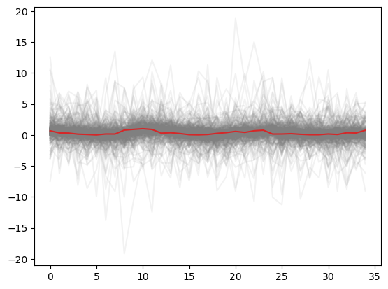
Again it is taking hours and hours to sample. Both prior predictive look great.
How can I improve the models above? Or even how sould I implement this kind of model?

1 Like

Your 2nd implementation looks great. Try using a JAX sampler with the following changes:

from pymc.pytensorf import collect_default_updates, get_mode
with pm.Model() as model:
    # priors...
    [l, b, y_hat], updates = scan(fn=step,
                                    sequences=[{'input':y_obs, 'taps':[0]}],
                                    outputs_info=[l0, b0, None],
                                    non_sequences=[alpha, beta, phi, sigma],
                                    strict=True, mode=get_mode('JAX'))
    obs = model.register_rv(y_hat, name='obs', observed=y_obs)
    idata = pm.sample(nuts_sampler='numpyro')

You can also play with passing nuts_sampler_kwargs=dict(chain_method = 'vectorized'} or chain_method='parallel' to pm.sample. I sometimes get faster results with one and sometimes faster with the other.

Also it’s recommended to avoid using the model.register_rv API, since it’s not guaranteed to be maintained going forward. The new way is to use pm.CustomDist, passing a function that returns the results of your scan as the dist. For your model, it would look like this:

from pymc.pytensorf import collect_default_updates, get_mode

def step(*args):
    y_tm1, l_tm1, b_tm1, alpha, beta, phi, sigma = args
    
    l = alpha * y_tm1 + (1 - alpha) * (l_tm1 + phi * b_tm1) # update the level
    b = beta * (l - l_tm1) + (1 - beta) * phi * b_tm1 # update the trend

    mu = l + phi * b # forecast
    y = pm.Normal.dist(mu=mu, sigma=sigma)
    
    return (l, b, y), collect_default_updates(inputs=args, outputs=[y]) 
    
def holt_winters(alpha, beta, phi, sigma, l0, b0, size, mode='JAX'):
        
    (l, b, y), updates = pytensor.scan(fn=step,
                                           sequences=[y_obs],
                                           outputs_info=[l0, b0, None],
                                           non_sequences=[alpha, beta, phi, sigma],
                                           strict=True, 
                                           n_steps=size[0],
                                           mode=get_mode(mode))
    
    return y
    
with pm.Model() as model:
    # Observed Data
    y_obs =  pm.MutableData('y_obs', Y)

    alpha = pm.Uniform('alpha', 0, 1)
    beta = pm.Uniform('beta', 0, 1)
    phi = pm.Uniform('phi', 0.8, 0.98)
    sigma = pm.HalfNormal('sigma', 0.1) # variance
    
    l0 = pm.Normal('l0', 0, 0.1) # initial level
    b0 = pm.Normal('b0', 0, 0.1) # initial trend
        
    y_pred = pm.CustomDist('obs', alpha, beta, phi, sigma, l0, b0, dist=holt_winters, observed=y_obs) 
    idata = pm.sample(nuts_sampler='numpyro', nuts_sampler_kwargs={'chain_method':'vectorized'})
1 Like

Nice! I really appreciate your answer!

Sorry for the delayed response Numpyro was kind hard to install on Apple Silicon.
Now I have a new problem. After changing to pm.CustomDist, I am no longer able to sample prior predictive or even posterior predictive.

TypeError: Cannot interpret value of type <class 'numpy.random._generator.Generator'> as an abstract array; it does not have a dtype attribute
Apply node that caused the error: Composite{...}(*5-<Scalar(float64, shape=())>, *2-<Scalar(float64, shape=())>, *1-<Scalar(float64, shape=())>, *7-<Scalar(float64, shape=())>, *0-<Scalar(float64, shape=())>, *8-<Scalar(float64, shape=())>, *4-<Scalar(float64, shape=())>)
Toposort index: 0
Inputs types: [TensorType(float64, shape=()), TensorType(float64, shape=()), TensorType(float64, shape=()), TensorType(float64, shape=()), TensorType(float64, shape=()), TensorType(float64, shape=()), TensorType(float64, shape=())]
Inputs shapes: [(), (), (), 'No shapes', (), (), (), (), ()]
Inputs strides: [(), (), (), 'No strides', (), (), (), (), ()]
Inputs values: [array(0.04778321), array(-0.1229446), array(0.09235863), Generator(PCG64) at 0x1691A9460, array(0.55552896), array(0.8099783), array(0.10233593), array(0.94326862), array(0.3600119)]
Outputs clients: [['output'], [normal_rv{0, (0, 0), floatX, False}(*3-<RandomGeneratorType>, [], 11, Composite{...}.1, *6-<Scalar(float64, shape=())>)], ['output']]

HINT: Re-running with most PyTensor optimizations disabled could provide a back-trace showing when this node was created. This can be done by setting the PyTensor flag 'optimizer=fast_compile'. If that does not work, PyTensor optimizations can be disabled with 'optimizer=None'.
HINT: Use the PyTensor flag `exception_verbosity=high` for a debug print-out and storage map footprint of this Apply node.
Apply node that caused the error: Scan{scan_fn, while_loop=False, inplace=all}(Shape_i{0}.0, Mul.0, SetSubtensor{:stop}.0, SetSubtensor{:stop}.0, RandomGeneratorSharedVariable(<Generator(PCG64) at 0x1691A9460>), Shape_i{0}.0, beta, phi, sigma, Sub.0, Composite{((i0 - i1) * i2)}.0)
Toposort index: 24
Inputs types: [TensorType(int64, shape=()), TensorType(float64, shape=(None,)), TensorType(float64, shape=(1,)), TensorType(float64, shape=(1,)), RandomGeneratorType, TensorType(int64, shape=()), TensorType(float64, shape=()), TensorType(float64, shape=()), TensorType(float64, shape=()), TensorType(float64, shape=()), TensorType(float64, shape=())]
Inputs shapes: [(), (36,), (1,), (1,), 'No shapes', (), (), (), (), (), ()]
Inputs strides: [(), (8,), (8,), (8,), 'No strides', (), (), (), (), (), ()]
Inputs values: [array(36), 'not shown', array([-0.1229446]), array([0.09235863]), Generator(PCG64) at 0x1691A9460, array(36), array(0.55552896), array(0.8099783), array(0.10233593), array(0.94326862), array(0.3600119)]
Outputs clients: [[], [], ['output'], ['output']]

HINT: Re-running with most PyTensor optimizations disabled could provide a back-trace showing when this node was created. This can be done by setting the PyTensor flag 'optimizer=fast_compile'. If that does not work, PyTensor optimizations can be disabled with 'optimizer=None'.
HINT: Use the PyTensor flag `exception_verbosity=high` for a debug print-out and storage map footprint of this Apply node.

Should I sample from the posterior by my own? How can I use the already implemented methods from Pymc?

Just to you to be able to test here is the Y value that I am using:

Y = np.array([0.84227129, 0.66561514, 0.32176656, 0.29652997, 0.12302839,
       0.06624606, 0.        , 0.14826498, 0.14195584, 0.77287066,
       0.89589905, 1.        , 0.87697161, 0.28391167, 0.3533123 ,
       0.22397476, 0.03470032, 0.0126183 , 0.06624606, 0.24921136,
       0.36908517, 0.56466877, 0.40063091, 0.66561514, 0.76025237,
       0.13880126, 0.14511041, 0.20189274, 0.0977918 , 0.03154574,
       0.03154574, 0.14826498, 0.06624606, 0.3533123 , 0.30914826,
       0.74763407])

What version of pymc/pytensor are you using? This is an area of the code base that is in super active development, so you need to be on the latest release

pymc.__version__ == '5.5.0'
pytensor.__version == '2.12.3'

This is definitely a bug. Could you open an issue on Github?

Can you confirm the following works as well:

    from functools import partial
    y_pred = pm.CustomDist('obs', alpha, beta, phi, sigma, l0, b0, dist=partial(holt_winters, mode=None), observed=y_obs) 
     prior = pm.sample_prior_predictive()

OK I worked a bit more on this. The key is that when you’re in JAX mode, you need to let the prior and posterior sampling functions know you’re using JAX. You do this by passing compile_kwargs=dict(mode=get_mode('JAX')) to all of your forward sampling functions.

There are a couple other small wrinkles.:

  1. You also cannot use pm.MutableData in JAX mode, because JAX needs to know all shapes at compile time (although PyMC could just re-compile each time you call pm.set_data, so I sort of consider this a bug). EDIT: You can use you it in general, but it fails here – something kind of interaction with scan is my guess.

  2. You need to make two y variables: one as y_obs[1:] and one as y_obs[:-1]. The first one is your observed data, because you can’t make a prediction about the first datapoint unless you also model y_{t-1} as an RV. The 2nd one is the lagged values you scan over.

  3. Finally, I also found a bug with pm.HalfNormal in JAX mode, so I changed the prior to Exponential.

Making all these changes, I ended up with the following code:

import jax
import pymc as pm
import arviz as az
import numpy as np

jax.config.update('jax_platform_name', 'cpu')
from pymc.pytensorf import collect_default_updates, get_mode
import pytensor 
from functools import partial


Y = np.array([0.84227129, 0.66561514, 0.32176656, 0.29652997, 0.12302839,
       0.06624606, 0.        , 0.14826498, 0.14195584, 0.77287066,
       0.89589905, 1.        , 0.87697161, 0.28391167, 0.3533123 ,
       0.22397476, 0.03470032, 0.0126183 , 0.06624606, 0.24921136,
       0.36908517, 0.56466877, 0.40063091, 0.66561514, 0.76025237,
       0.13880126, 0.14511041, 0.20189274, 0.0977918 , 0.03154574,
       0.03154574, 0.14826498, 0.06624606, 0.3533123 , 0.30914826,
       0.74763407])

def step(*args):
    y_tm1, l_tm1, b_tm1, alpha, beta, phi, sigma = args
    
    l = alpha * y_tm1 + (1 - alpha) * (l_tm1 + phi * b_tm1) # update the level
    b = beta * (l - l_tm1) + (1 - beta) * phi * b_tm1 # update the trend

    mu = l + phi * b # forecast
    y = pm.Normal.dist(mu=mu, sigma=sigma)
    
    return (l, b, y), collect_default_updates(inputs=args, outputs=[l, b, y]) 
    
def holt_winters(lagged_data, alpha, beta, phi, sigma, l0, b0, size, mode='JAX'):
        
    (l, b, y), updates = pytensor.scan(fn=step,
                                       sequences=[lagged_data],
                                       outputs_info=[l0, b0, None],
                                       non_sequences=[alpha, beta, phi, sigma],
                                       strict=True, 
                                       n_steps=size[0],
                                       mode=get_mode(mode))
    
    return y

def make_model(data, mode=None):    
    with pm.Model() as model:
        # Observed Data
        y_obs =  pm.ConstantData('y_obs', data[1:])
        y_lagged = pm.ConstantData('y', data[:-1])

        alpha = pm.Uniform('alpha', 0, 1)
        beta = pm.Uniform('beta', 0, 1)
        phi = pm.Uniform('phi', 0.8, 0.98)
        sigma = pm.Exponential('sigma', 1) # variance

        l0 = pm.Normal('l0', 0, 0.1) # initial level
        b0 = pm.Normal('b0', 0, 0.1) # initial trend

        y_pred = pm.CustomDist('obs', y_lagged, alpha, beta, phi, sigma, l0, b0, 
                               dist=partial(holt_winters, mode=MODE), 
                               observed=y_obs) 
    return model

MODE = 'JAX'
compile_kwargs={'mode':get_mode(MODE)}
sampler_by_mode = {'JAX':'numpyro', 'NUMBA':'nutpie', None:'Pymc'}

with make_model(Y, mode=MODE):
    prior = pm.sample_prior_predictive(compile_kwargs=compile_kwargs)
    idata = pm.sample(nuts_sampler=sampler_by_mode[MODE], 
                      nuts_sampler_kwargs={'chain_method':'vectorized'})
    idata = pm.sample_posterior_predictive(idata, 
                                           extend_inferencedata=True, 
                                           compile_kwargs=compile_kwargs)

Prior:
image

Posterior:
image

Estimates:

        mean     sd  hdi_3%  hdi_97%  mcse_mean  mcse_sd  ess_bulk  ess_tail  r_hat
l0     0.009  0.098  -0.178    0.195      0.001    0.002    4840.0    3018.0    1.0
b0    -0.048  0.090  -0.209    0.128      0.002    0.001    3567.0    2635.0    1.0
alpha  0.850  0.103   0.669    0.999      0.002    0.001    3325.0    2328.0    1.0
beta   0.166  0.187   0.000    0.549      0.004    0.003    2925.0    2118.0    1.0
phi    0.870  0.049   0.800    0.958      0.001    0.001    4001.0    2684.0    1.0
sigma  0.256  0.034   0.199    0.323      0.001    0.000    4585.0    3115.0    1.0
2 Likes

@Cristianobam @jessegrabowski

When I study this case, I have some questions.

  1. In the pytensor.scan, why y_obs is a sequence?
  2. What is the meaning of y = pm.Normal.dist(mu=mu, sigma=sigma)? I mean, we have the observed data, and we already use pm.CustomDist to generate logp. Why do we have to define the distribution of y. Why we can’t just use the observed data to fit mu here?

Any reply will be appreciated very much.

y_obs is a sequence because it’s a distribution over one-step-ahead predictions. You might be able to write it without this, by just running for n_steps, but I think the noise would overwhelm the signal. If you try it please report back!

The forecast, y, is itself a random variable. The forecast is not just a mean, it’s a distribution over values at the next time step. The CustomDist will infer the logp of the scan, but it needs to include all the sources of randomness from the model.