Hi Milton, I also just finished my undergrad and worked on a Bayesian SIR-like model so I can give you some (hopefully) useful pointers given my experience.
The first thing I noticed in your notebook is that you are modeling the cumulative mortalities with a Normal likelihood. In my model and in the others I have read about, people try to fit their models to the number of daily new mortalities rather than the daily cumulative mortalities. I originally did what you did and ran into similar issues with sampling. The way I reason about it is that it doesn’t seem reasonable to observe the cumulative mortalities curve with the same absolute level of noise throughout the pandemic… you’d expect this to scale with the total number of deaths. Fitting the model to daily mortalities is one way to accomplish this.
Whenever I run into issues like this, I like to look at the posterior predictive distribution… sometimes this can be helpful with figuring out why your model is giving bogus results. You can sample the posterior predictive distribution with pm.sample_posterior_predictive():
with model:
    ppc = pm.sample_posterior_predictive(trace)
When I do this with the model in your notebook and plot the results, I get the following:

This certainly isn’t right - samples from the posterior predictive in your case should each look like draws of the cumulative death curves (with normal noise). So this means that your model as coded isn’t doing what you think it is. I threw in a pm.Deterministic() to track the mortality dimension of your sir_curves variable directly, and found that the samples looked like this:

This is your first hint. The posterior predictive looks unruly while your de-noised mortality curves don’t look too bad, so let’s try turning the noise in your likelihood way down and also let it be an inferred parameter. You currently have sigma=1 in your likelihood… this leads to a huge variance compared to the size of your data, which lies between 0 and 1 (since compartments sum to 1). Let’s see what happens to the posterior predictive distribution and the de-noised mortality curves:
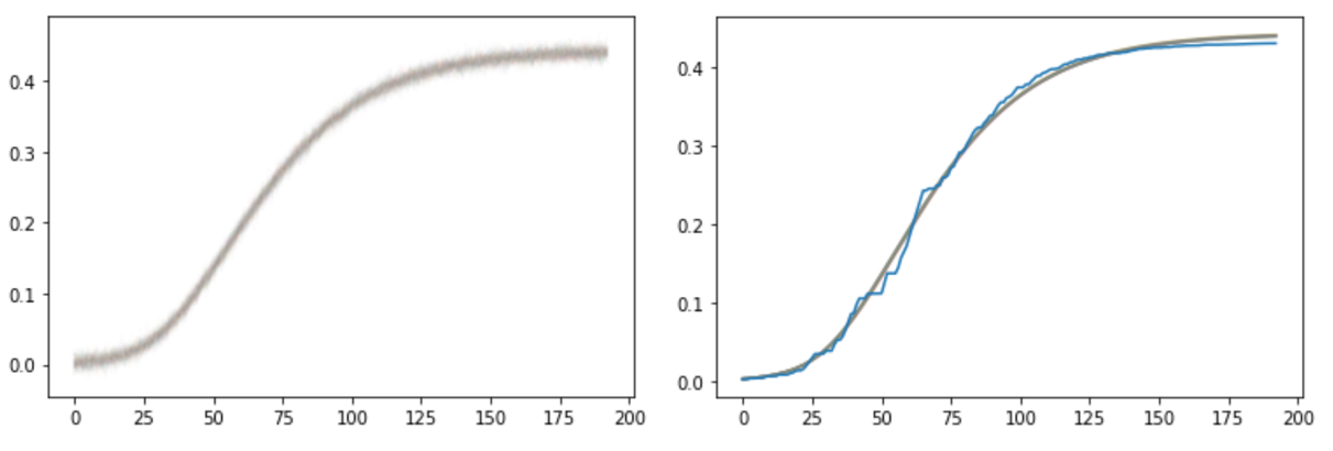
So this is much better. However, when I take a look at the posteriors for R0 and a, I see that they’re now much thinner but seem to be centered a bit away from the true values in your notebook. My initial hypothesis is that this is being caused due to the fact that you’re enforcing a normal likelihood on the cumulative mortality curve rather than on the daily increments of this curve - in some sense, a better fitting model lies outside the “span” of your current setup. However, I switched your model to fit on the daily increments and it seemed to perform comparably… so I may be wrong on this. I think you also have an issue going on with the way you treat the interpolation. When you truncate your data, you truncate the mortality data from the front while you truncate the time vector from the back… I think this is what’s causing you to infer R0 and a incorrectly. My suggestion would be to try changing
day0 = 275
D_obs = D_obs[day0:]
y0 = y[day0, :]
days = len(D_obs)
t = np.linspace(0, days-1, days)
to
day0 = 275
D_obs = D_obs[day0:]
y0 = y[day0, :]
days = len(D_obs)
t = np.linspace(day0, day0+days-1, days)
p.s. Some models I recommend taking a look at are the Prieseman group’s model (written in PyMC!) and the MechBayes model.