Best way to plot and do PPC with variable that has (too) many levels

Thank you all for developing this amazing package! I’m having a hard time selecting levels of a factorial variable to plot. For example, instead of 8 schools, we assume there are 48 schools in total.

%matplotlib inline
import pymc3 as pm
import numpy as np
import matplotlib.pyplot as plt
plt.style.use('seaborn-darkgrid')

J = 48
y = np.array([ 28,   8,  -3,  7, -1,  1,  18,  12,
               -2,  15,  12,  5,  9,  1,  34,   6,
                4,  23,  -6, -3, 19,  2,   8,  10,
               17,  -2,   4,  1, 13,  21,  3,   2,
                3, -10,   1,  7,  27, -1,  6,   9,
               -4,  5,   13, 25, -12,  7,  2,  19])
sigma = np.array([15, 10, 16, 11, 9, 11, 10, 18,
                  13, 20, 7, 11, 12, 9, 16, 10,
                  16, 8, 20, 17, 19, 11, 15, 12,
                  10, 19, 20, 13, 12, 18, 16, 18,
                  9, 14, 11, 10, 18, 20, 7, 14,
                  7, 11, 22, 19, 20, 18, 11, 10])

with pm.Model() as hierarchical:

    eta = pm.Normal('eta', 0, 1, shape=J)
    mu = pm.Normal('mu', 0, sd=1e6)
    tau = pm.HalfCauchy('tau', 5)

    theta = pm.Deterministic('theta', mu + tau*eta)

    obs = pm.Normal('obs', theta, sd=sigma, observed=y)

    trace_h = pm.sample(1000)

pm.forestplot(trace_h, varnames=['theta']);

pm.plot_posterior(trace_h, varnames=['theta'], color='#87ceeb');

My questions are as follows:

  • How do I select only thetas with level 10-20 and plot the trace (forestplot, parallel coordinate plot, plot_posterior)?
  • How do I tune the size of the forestplot?
  • I have tried arviz for this as well. Is there also a solution currently to tune the plot size of arviz?

Thanks again!

I would index to the trace and select the slice, but maybe @colcarroll and @aloctavodia knows a more native solution in arviz

Oh boy! With ArviZ, this is pretty straightforward. The only tricky part is remembering how to name a dimension:

data = az.from_pymc3(
    trace=trace_h, 
    coords={'school': range(J)}, 
    dims={'eta': ['school'], 'theta': ['school'], 'obs': ['school']}
)

after that, all the plots you asked for are quite pleasant (if we passed a list of J strings instead of range(J) to the coords argument, we could have even nicer labels):

az.plot_trace(data, var_names='theta', coords={'school': range(10, 20)});
az.plot_forest(data.posterior.sel(school=range(10, 20)), var_names='theta');
az.plot_parallel(data, var_names='theta', coords={'school': range(10, 20)});
az.plot_posterior(data, var_names='theta', coords={'school': range(10, 20)});

Notice that we forgot to have a coords argument for the forest plot, but you can work around that using xarray slicing! plot_forest takes a figsize argument as well:

az.plot_forest(data.posterior.sel(school=range(10, 20)), var_names='theta', figsize=(9, 6));

image

5 Likes

Thanks for your help @colcarroll @junpenglao. I tried the arviz coords method before, but ran into an error on y_max() inside forestplot. Not sure what caused that. However, it worked after reinstalling arviz from git master. Thanks again!

Hello, and first of all, many thanks for a beautiful tool, PYMC3! I just recently migrated from version 2, and I’m absolutely flabbergasted over how powerful and user friendly 3 is…!

Now, I’m trying to learn all the cool new capabilities. In particular, I’m trying to figure out how to use the coords-feature for a model with varying intercepts and slopes.

Perhaps easiest to express my question is by providing simple example code:

import numpy as np
import pandas as pd
import matplotlib.pyplot as plt
import seaborn as sns
import pymc3 as pm
import arviz as az

sns.set()

df = pd.read_csv(‘https://raw.githubusercontent.com/tolex3/resources/master/Rethinking_2/Data/Howell1.csv’,sep=’;’)

df.head()

df = df.loc[df[‘age’] >= 18]
df.plot(x=‘weight’,y=‘height’,kind=‘scatter’,color=‘b’)

x = df[‘weight’].values
gender_idx = df[‘male’]

model = pm.Model()
with model:
alpha = pm.Normal(‘alpha’,170,30,shape=2)
beta = pm.Normal(‘beta’,1,2,shape=2)
sigma = pm.Uniform(‘sigma’,0,50)

reg = pm.Deterministic('reg',alpha[gender_idx] + beta[gender_idx] * x)

obs = pm.Normal('obs',mu=reg,sd=sigma,observed=df['height'])

trace = pm.sample(500,tune=500)

with model:
idata = az.from_pymc3(trace,coords={‘gender_idx’: np.array([‘female’,‘male’])},
dims={‘alpha’: [‘gender_idx’], ‘beta’: [‘gender_idx’]})

_ = az.plot_posterior(idata,var_names=['alpha','beta'],
                      coords={'gender_idx' : ['female','male']},
                     figsize=(18,12))

plt.plot(x,trace[‘alpha’][:,0].mean() + x * trace[‘beta’][:,0].mean(),color=‘crimson’,ls=‘dashed’)
plt.plot(x,trace[‘alpha’][:,1].mean() + x * trace[‘beta’][:,1].mean(),color=‘navy’,ls=‘dashed’)

ax = plt.gca()

draws = range(0,len(trace[‘reg’]),10)

plt.plot(x,trace[‘alpha’][:,1][draws] + trace[‘beta’][:,1][draws] * x[:,None],color=‘lightblue’,alpha=0.05)
_ = plt.plot(x,trace[‘alpha’][:,0][draws] + trace[‘beta’][:,0][draws] * x[:,None],color=‘orange’,alpha=0.05)

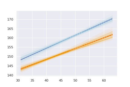
QUESTION : HOW TO DO THE below TWO CI-PLOTS WITH ARVIZ ?

that is, how to make arviz ‘aware’ which of the items in trace[‘reg’] belong to the male/female categories ?

az.plot_hdi(x,trace[‘reg’],ax=ax) ???

how should I write the coords/dims argument above to be able to use az.plot_hdi for the below plot ?

arviz_question

thanks,
Tommy

figured out another way to accomplish what I want, using az.plot_hdi: by manually extracting the x,y coordinates for male/female from the df and trace, respectively:

f_idx = df[‘male’] == 0
m_idx = df[‘male’] == 1

x_f = df.loc[df[‘male’] == 0][‘weight’]
x_m = df.loc[df[‘male’] == 1][‘weight’]

trace_f = trace[‘reg’][:,f_idx]
trace_m = trace[‘reg’][:,m_idx]

az.plot_hdi(x_f,trace_f,ax=ax)
az.plot_hdi(x_m,trace_m,ax=ax)

arviz_question

But I’m sure there’s a better way doing this…?

1 Like

Hi @tolex3, welcome!

I’d recommend using arviz.InferenceData and xarray to simplify your code and get automatic broadcasting. The Primer on Bayesian Methods for Multilevel Modeling example is a good example about how to use them in situations very close to yours and I think will be useful.

Now moving to your particular case.

There is no need to use the coords argument here, the default is to generate a subplot for each coordinate value. You’d need to use something like coords={"gender_idx": ["female"]} to plot only one of the two cases.

Following what is done in the example notebook above, I’d go for a similar approach here. We can start by storing the results in a new variable mu and then use it for plotting:

x_da = xr.DataArray(x, dims=["x_idx"])
mu = idata.posterior["alpha"] + x_da * idata.posterior["beta"]
# I think this should be equivalent to 
mu = idata.posterior["reg"]

to get xarray to take care of the broadcasting, all terms have to be xarray objects so I create x as a DataArray. You can also read this blogpost to get ArviZ to store x and skip this step. You’d then access x_da as idata.constant_data["x"].

_, ax = plt.subplots()
ax.plot(x, mu.mean(("chain", "draw")).sel(gender_idx="female"), color="crimson", ls="--")
ax.plot(x, mu.mean(("chain", "draw")).sel(gender_idx="male"), color="navy", ls="--")
ax.plot(
    x, 
    mu.sel(gender_idx="male", draw=slice(None, None, 10)), 
    color=‘lightblue’,
    alpha=0.05
)
ax.plot(x, mu.sel(gender_idx="male", draw=slice(None, None, 10)),color=‘orange’,alpha=0.05)

The code to select the subset of the data we are interested in is now slightly longer, but mostly because it’s more explicit, with xarray we can operate and select using named labels. Thanks to this I think that the code is mostly self explainatory.

Now to hdi. I think here it’s best to use the hdi_data argument of plot_hdi. I would start computing the hdi, and then plotting each gender:

mu_hdi = az.hdi(mu)["mu"]
_, ax = plt.subplots()
az.plot_hdi(x, hdi_data=mu_hdi.sel(gender_idx="male"), ax=ax)
az.plot_hdi(x, hdi_data=mu_hdi.sel(gender_idx="female"), ax=ax)

Note: All these plots are showing the distribution and values of the observed mean which is not the same as the distribution of the posterior predictive values.

I hope it helps!

3 Likes

Hi Oriol, and “wow!” for your elaborate answer! I’ve been lurking here for some time, and from start been very impressed by the quality of the answers provided, as well as by the patience of those answering… :slight_smile:

I will look into all the suggestions you make in your reply - no doubt will it take me a few days to “chew” and trying to understand all of it, but rest sure I will put the necessary effort into it, and eventually let you know whether I “got it”… :slight_smile: Again, many thanks for your reply and a beautiful tool!
cheers,
Tommy

1 Like