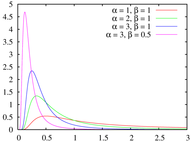
I have a dataset with a pdf like in the attached image. There is a lower limit of detection on my measured data, but it doesn’t take on a precise value, hence the spike in data is a narrow distribution, but not a line. Instead of the data being censored, I have a lot of values close to the limit of detection. I assume there is some normal distribution in reality, that is being “truncated” by my measurement.
How would I deal with this in PyMC3? I’ve explored the bounded and truncated distributions, but those seem to deal moreso with censored data? There’s information contained in the proportion of the pdf that is in the limit of detection region, so I’d rather not just censor it. Thoughts?
Thanks for the quick suggestion. I’ll give it a shot, but looking at the example curves in your link, I’m thinking skewnormal may be to “soft” a curve to fit such a hard shoulder in my data. The cartoon I drew, is actually a generous representation. A kde of my data looks about like a 90deg angle, with 90% of the data in the narrow, limit of detection peak, and 10% of it in the tail of the normal distribution that it’s truncating.
To clarify: I think that the true values of my data follow the dashed red curve (or something like it), but due to my limit of detection, my observed pdf is the blue curve. I’d like to infer mu_actual (it’s actually a variable that I’m regressing and has physical meaning to it). Hence I would need some sort of unimodal distribution, where the mode would be below the limit of detection region, despite the data showing a mode at the limit of detection region.
Hey Chris - that definitely comes closer to the steepness I need, but not sure it fits the end goal, as I’m hoping to estimate a physical parameter with true value on the unobserved side of the limit of detection. Hopefully that makes sense. I dropped a new graphic out in the parent thread to show what I mean.
This might be going out on a limb here but do you have any rough idea of the process that maps the true value to the observed one? For example, if there was a specific nonlinear function that we could build in.
I have an idea of the physical process, but unfortunately not something that could be mapped by 1:1 function I don’t think. Basically, the “x” value that is measured is a microbial density (CFU/mL or colony forming units of microbes per milliliter of sample). This is a log scale, and if you take a big enough volume (many liters) you’ll always find a colony forming unit when you culture the sample. However, in practice, the lab samples progressively larger volumes to count the microbes, but only looks down to ~1 CFU/mL and does not sample larger volumes to see if it might have been 0.1CFU/mL. So everything below 1-1.5 CFU/mL maps to 1-1.5 CFU/mL.
My suspicion is that we would have to make some very specific parametric assumptions regarding how the probability mass to the left of the detection limit gets transferred to the vicinity of the limit. Could we perhaps model it as censored data plus some additive positive noise that is an increasing function of \mu_{actual} over some region close to the detection limit?
Just to close this out: I found that the topic I needed was data ‘censoring’. There are several helpful threads online addressing censoring in bayesian (and specifically pymc3) models. Conceptually, I simply integrated the probability mass below my censoring limit, and accounted for this with the pm.potential function. There are built-in functions for this, and plenty of coverage online, just needed to know what to search for: ‘tobit regression’, ‘data censoring’, ‘truncated vs. censored’, etc. Hope this is helpful to anyone else having this issue. The solution worked quite well, and made a big difference in model quality.
Censoring should work fine. Another idea that you could try is to explicitly model a “background” value of some sort. I don’t know what the context is, but I had issues like this a couple of times with measurements of concentrations, where your always measure at least some background value even if the true concentration were 0. If we model the log-concentrations we get something like:
log_background = pm.Normal('log_background', mu=-2, sd=0.1)
# Say, a regression for the actual log_concentration
log_concentration = (
    intercept
    + foo
    + bar
)
log_mu = pm.math.logaddexp(log_concentration, log_background)
pm.Normal('log_measured', mu=log_mu, observed=data)
Worked pretty well for me, but might not make sense in your setting of course…

