PyMC Syntax Explainer: Why the Sausage is Made like This?

Hello everyone,

I’m a beginner to PyMC and am quickly learning a lot but I’m struggling to generalize the code snippets found in the Example page.

The website has been immensely helpful to learn by example, but I feel like I’m missing a deeper understanding. As I’m branching out on my own I realize I don’t understand how these lines of code connect to each other from an implementation perspective. From trial and error I can fix most of my mistakes but I don’t know WHY these mistakes cause problems with PyMC. Many of my problems are because I’ve given PyMC the correct information, just in the wrong place or in the wrong order for what I want it to do.

Can you all suggest a resource that describes how PyMC works under the hood?

I suspect I will figure this out in time, but I want to see if there’s something that can help me along as I get there. Thank you in advance!

1 Like

Welcome!

It can definitely be a bit confusing where all the little bits are specified. Can you give some examples of things you have stumbled over? That might help someone provide some pointers to resources that might help.

Thank you for your response! My most recent problem is a two connected hierarchical models, small dataset here:

School,StudentID,RepeatID,science_test1,science_test2
Jefferson,A,First Try,98.63,96.24
Jefferson,A,Second Try,99.35,109.69
Jefferson,A,Third Try,102.06,94.72
Jefferson,B,First Try,102.75,102.53
Jefferson,B,Second Try,104.93,97.91
Jefferson,B,Third Try,92.75,99.62
Jefferson,C,First Try,108.93,131.58
Jefferson,C,Second Try,98.98,88.41
Jefferson,C,Third Try,92.75,85.96
Jefferson,D,First Try,109.99,120.98
Jefferson,D,Second Try,91.21,85.17
Jefferson,D,Third Try,99.68,97.05
Washington,E,First Try,9.05,3.7
Washington,E,Second Try,0.46,0.85
Washington,E,Third Try,0.68,1.69
Washington,F,First Try,0.15,0.2
Washington,F,Second Try,0.75,0.8
Washington,F,Third Try,0.43,0.46
Washington,G,First Try,1.24,1.35
Washington,G,Second Try,0.7,1.11
Washington,G,Third Try,1.58,1.49
Washington,H,First Try,7.5,0.5
Washington,H,Second Try,0.59,0.49
Washington,H,Third Try,0.43,0.47

I want to test if there is a difference in scientific ability between the Jefferson school and the Washington school as measured by both of the science tests (NOTE: in the full dataset there are more than 2 schools). In each of the 2 schools each of 4 students takes each of 2 tests 3 different times. I am able to estimate one beta for each school-test pair and pool into two betas one level above the test level:

image

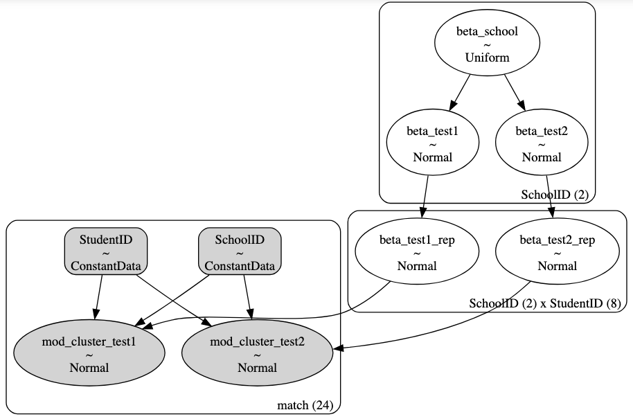
But this model doesn’t cluster scores at the StudentID level and that clustering is what I am struggling with. I want to estimate a model like this:

I think I’m encoding the hierarchy correctly but something is going wrong with how I’m giving PyMC the indicators for SchoolID and StudentID and I don’t understand why. When I try to sample this model it gives a ValueError: Incompatible Elemwise input shapes.

How does this clustering work with PyMC? In the final model call I’m telling PyMC to cluster by school and student by subsetting a pm.Normal object like:

mod_test1 = pm.Normal("mod_cluster_test1",
                      mu = beta_test1_rep[school, student],
                      sigma = 2,
                      observed = df.science_test1,
                      dims = "match")

But I suspect this is incorrect, or at least not flexible enough. It’s only this one model that’s going wrong because I’ve done this double subsetting before and it’s worked just fine. Perhaps I’ve encoded something else wrong in this model?

1 Like

I guess I have 2 suggestions, one of which is a very narrow approach to try and address this specific example and one of which is a broader approach to hierarchical modeling.

  1. (narrow) The mu in your likelihood (beta_test1_rep[school, student]) should be the same shape as the observed data you are connecting that likelihood to (df.science_test1). Without seeing a lot more of your code, it’s unclear that these shapes match, but the error you are seeing suggests a mismatch somewhere along the line.
  2. (broad) I would probably work through some relatively basic examples of hierarchical models to get a feel for how adding new levels works in general. The multi-level modeling notebook is pretty good at contrasting the hierarchical model with each of 2 (possibly more) intuitive counterparts. Or you can spin through one of the textbooks and their coverage/explanation/tutorials on building hierarchies. I tend to rely on this chapter from Kruschke’s Doing Bayesian Data Analysis.

Thank you for the narrow suggestion, I will look into this!

On the broad comment I have read that chapter from Krushke (and the PyMC code port on GitHub) and I have worked through the Radon example and the Rugby example in PyMC. My lack of understanding stems from how these examples encode the hierarchy of the model using different syntax and I cannot find explanations of how each syntax works.

The Radon example and the DBDA PyMC3 notebook uses a formula-like syntax:

alpha[county_idx] + beta * floor_idx

But the Rugby example only uses a subset-like syntax:

intercept + atts[away_idx] + defs[home_idx]

From the examples both of these syntaxes get to the goal but it’s unclear when is appropriate to use one or when to use the other and how each one generalizes to my double hierarchy use case.

The differences you are seeing in these two examples represent substantive differences in how the models are constructed. In the first case

alpha[county_idx] + beta * floor_idx

the model is a varying-intercept model, in which each there is a separate alpha for each county. There are 85 counties (so alpha is an array with 85 entries in it), but the data has 919 observations. To get a mean (mu) for each of the corresponding 919 observations, you need to generate a vector of 919 means, each of which requires the corresponding alpha. So county_idx is a vector of indices, specifying which observation corresponds to which county. Similarly, floor_idx encodes which floor each observation corresponds to. However, the effect of “floor” is identical, regardless of which county the observation is taken from. So, the effect of “floor” is just beta*floor_idx.

In the second case

atts = pm.Deterministic("atts", atts_star - pt.mean(atts_star), dims="team")
defs = pm.Deterministic("defs", defs_star - pt.mean(defs_star), dims="team")
home_theta = pt.exp(intercept + home + atts[home_idx] + defs[away_idx])
away_theta = pt.exp(intercept + atts[away_idx] + defs[home_idx])
...

there is a separate value of atts for each team a separate value of defs for each team (note the dims="team" in the creation of each). But, like above, we need a value of home_theta (and away_theta) for each match recorded in our observed data. So we need a way to map the set of atts to their corresponding observations. We do so, by creating away_idx which allows us to select the appropriate values of atts for each observation. In this model, there is a single intercept that does not vary by team, so it’s just a single value, intercept.

Hopefully that helps you get a bit farther along in your journey!

2 Likes

If you are just starting I suggest you follow McElreath book/class (it’s on YouTube) Statistical Rethinking and the corresponding PyMC port of the examples. He will gradually introduce hierarchical models. It’s a slower process but a less steep one

1 Like