Hierarchical regression models for ratings data ( 2 by 2 within-subject design)

[hcp4715]

Dear there,

I am trying to use Bayesian hierarchical regression models (or Bayesian linear mixed model) to analyze a small dataset that we usually do with repeated-measure ANOVAs. I could have run it using BRMs, but I decide to use PyMC3 because I think PyMC3 will force me to learn the details about constructing a model. However, I am new to Bayesian hierarchical/multi-level models, so I am trying my best to describe my question. If you feel that my description is not clear enough, please point it out, and I will add more info.

My data are from 25 participants’ subjective ratings in a 2 by 2 within-subject design (i.e., 4 conditions in total). Each participant has 4 ratings for each condition (i.e., 16 ratings in total). The ratings are from 0 ~ 99, with many zeros for some conditions.

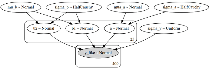
I first tried to follow this tutorial: https://docs.pymc.io/notebooks/multilevel_modeling.html. It worked well until I tried to include the interaction between two variables. So the last model I constructed is like this:

with Model() as example_LMM:
    
    # priors
    mu_a = Normal('mua_a', mu=0., sigma=1e5)
    sigma_a = HalfCauchy('sigma_a', 5)
    mu_b = Normal('mu_b', mu=0., sigma=1e5)
    sigma_b = HalfCauchy('sigma_b', 5)
    
    # Random intecepts
    a = Normal('a', mu=mu_a, sigma=sigma_a, shape=subjs)
    b1 = Normal('b1', mu=mu_b, sigma=sigma_b, shape=subjs)
    b2 = Normal('b2', mu=mu_b, sigma=sigma_b, shape=subjs)
    
    # Model error
    sigma_y = Uniform('sigma_y', lower = 0, upper=100)
    
    # expected value
    y_hat = a[subj] + b1[subj]*blockType + b2[subj]*CSType
    
    # Data likelihood
    y_like = Normal('y_like', mu=y_hat, sigma=sigma_y, observed=AnxRatings)
    
model_to_graphviz(example_LMM)

Then I read these two posts

Hierarchical Linear Regression Model -- why is it not converging?

I created a toy example: 5 Regions with x and y Data; 30 data-items each; Region 5 contains just one pair: N = 30 beta_0 = [3, 3.2, 2.4, 4.1] beta_1 = [11, 10, 9.1, 14.1] idx = np.repeat(range(4),N) x = np.array([]) ; y = np.array([]) for b_0,b_1 in zip(beta_0,beta_1): x_new = st.uniform(0,20).rvs(N) x = np.append(x, x_new) eps = st.norm(0,10).rvs(N) y = np.append(y,b_0 + b_1*x_new + eps) x = np.append(x,10) ; y = np.append(y,3+11*10) idx = np.append(idx,4) A non-hierarchical …

Constructing the random effects model matrix Z

I am trying to replicate the sleep deprivation study found in the R package LME4 (for fitting linear mixed effects models) and described in this paper. The dataset sleepstudy contains the average reaction time per day for subjects in a sleep deprivation study. On day 0 the subjects had their normal amount of sleep. Starting that night they were restricted to 3 hours of sleep per night. The observations represent the average reaction time on a series of tests given each day to each subject. W…

And I tried to imitate the model from the first one (thanks @Jack_Caster for sharing the notebook), and wrote a model like this:

(mx_en, mx_ex) = pt.dmatrices("AnxRating ~ blockType * CSType", data=df_d1, return_type='dataframe')
with Model() as mdl_interaction:
    
    # define priors weakly informative Normal
    # Fixed effects
    #mu_a = Normal('mua_a', mu=0., sigma=100)
    #sigma_a = HalfCauchy('sigma_a', 5)
    #mu_b = Normal('mu_b', mu=0., sigma=100)
    #sigma_b = HalfCauchy('sigma_b', 5)
    beta_X_intercept = pm.HalfNormal('beta_X_intercept', sd=1000) # contrain it to positive values
    beta1_X_slope = pm.Normal('beta1_X_slope', mu=0, sd=100)
    beta2_X_slope = pm.Normal('beta2_X_slope', mu=0, sd=100)
    beta3_X_slope = pm.Normal('beta3_X_slope', mu=0, sd=100)
    beta_X = tt.stack(beta_X_intercept, beta1_X_slope, beta2_X_slope, beta3_X_slope)
    
    estimate_X = pm.math.dot(X, beta_X)
    
    # Random intecepts
    #a = Normal('a', mu=mu_a, sigma=sigma_a, shape=subjs)
    #b1 = Normal('b1', mu=mu_b, sigma=sigma_b, shape=subjs)
    #b2 = Normal('b2', mu=mu_b, sigma=sigma_b, shape=subjs)
    #b3 = Normal('b3', mu=mu_b, sigma=sigma_b, shape=subjs)
    
    ## Random effect
    sigma_Z = pm.HalfNormal('sigma_Z', sd=100)
    gamma_Z_raw = pm.Normal('gamma_Z_raw', mu=0, sd=1, shape=Z.shape[1])
    gamma_Z = pm.Deterministic('gamma_Z', gamma_Z_raw * sigma_Z)
    
    estimate_Z = pm.math.dot(Z, gamma_Z) 
    
    
    # Model error
    #sigma_y = Normal('sigma_y', mu = 0, sigma=1e6)
    
    # expected value
    #y_hat = (a[subj] + 
    #        b1[subj]*mx_ex['blockType'] + 
    #        b2[subj]*mx_ex['CSType'] +
    #        b3[subj]*mx_ex['blockType:CSType'])
    
    mu_estimate = pm.Deterministic('mu_estimate', estimate_X + estimate_Z)
    sigma_unexplained = pm.HalfNormal('sigma_unexplained', sd=1000) # unexplained variability
    y_likelihood = pm.Normal('y_likelihood', mu=mu_estimate, sd=sigma_unexplained, observed=AnxRatings)
    
    # Data likelihood
    #y_like = Normal('y_like', mu=y_hat, sigma=sigma_y, observed=AnxRatings)
    
model_to_graphviz(mdl_interaction)

I also realized that the model from https://docs.pymc.io/notebooks/multilevel_modeling.html (let’s call this as example 1) and Hierarchical Linear Regression Model -- why is it not converging? (let’s call this as example 2) are different.

I felt that there are a few points that I am not very clear so that I need some guide, maybe just pointing to me where can I found the answer. These points are:

(1) If I understand correctly, example 2 includes both the fixed effect & random effect, example 1 only includes the random effect? I am a bit confusing: are we supposed to always include both fixed and random effect?

(2) For example 2 (Hierarchical Linear Regression Model -- why is it not converging?) and here (Constructing the random effects model matrix Z), the deterministic function were included, when should we use this?

(3) How to plot the traces of random effect together. I as saw @Jack_Caster’s note book (https://github.com/JackCaster/GLM_with_PyMC3/blob/master/notebooks/LME%20-%20Sleep%20study.ipynb), the trace of random effect gamma_Z were plotted together:

But when I tried to plot this notebook in my own PC, seems they are in different subplots.

(4) I knew that Normal distribution is not appropriate for my data (ratings), what would be a better choice?

Many thanks.

[AlexAndorra]

Hi there!
That’s a lot of questions – I don’t think I’ll be able to answer all of them but I’ll try to tackle some
First, some remarks:

• I think you didn’t say why you abandonned your first model (example_LMM): what kind of problem did you have there? This model seems nicely written to me – provided your data can be appropriately described by a normal likelihood. The thing I’d do though is:

  • Choose clearly more regularizing priors: a sigma of at most 10 for the mus and an Exponential instead of HalfCauchy or Uniform for the sigmas should be more appropriate for sampling and more scientifically justified – in any case, prior predictive checks would be useful here
  • I think you need different hyper parameters for your slope coefficients b1 and b2, because they come from two different statistical populations. Currently, you’re constraining your model to have the same mean slope for blockType and CSType.
  • If b1 and b2 are indeed intercepts and not slopes, as the comment in your code suggests, then their mean should be 0: the baseline effect is already taken into account by mu_a
  • If your first model answers your question, I’d use it instead of the second model (mdl_interaction), mainly because it’s much simpler and easier to read and share

Now for your questions:

@hcp4715

(1) If I understand correctly, example 2 includes both the fixed effect & random effect, example 1 only includes the random effect? I am a bit confusing: are we supposed to always include both fixed and random effect?

Yes, that’s the idea of varying-effects models (I prefer this term to random effects, they have the same meaning in this context): you model the population of clusters (fixed effects) at the same time as you model each individual cluster (varying effects). This allows pooling of information, which aims at guarding against underfitting and overfitting at the same time. This NB is a very good introduction to these kinds of models, from McElreath excellent book.

@hcp4715

(2) For example 2 (Hierarchical Linear Regression Model – why is it not converging?) and here (Constructing the random effects model matrix Z), the deterministic function were included, when should we use this?

Deterministic variables are entirely determined by other random variables (e.g the sum of 2 RVs). pm.Deterministic is a way to tell PyMC to include this variable in the trace, even if it’s not an RV – you often do that for variables of interest; here that could be y_hat.

@hcp4715

(3) How to plot the traces of random effect together.

Here I think you’re looking for the kwarg compact=True in ArviZ’s plot_trace function.

@hcp4715

(4) I knew that Normal distribution is not appropriate for my data (ratings), what would be a better choice?

Even though I think you didn’t share the data here, I think you’re right: if the observations are integers between 0 and 99, that could be hard to model with a Normal. Plus, I guess your ratings have an inherent order (e.g 99 is better than 0), which you should take into account. It also depends on your target of inference – what are you interested in? The effect of predictors on the probability of ratings in each of the four conditions?
I don’t have a lot of experience in ranked-data models, but maybe an ordered logistic likelihood could be interesting here? This NB shows how to implement these models in PyMC3 – again, taken from McElreath’s masterpiece

Hope this helps! Good luck and PyMCheers

[hcp4715]

Hi, @AlexAndorra,

Thanks a lot for your reply! I think you solved my questions (2) ~ (4), but I am still a bit confused about the first question.

@AlexAndorra

you model the population of clusters (fixed effects) at the same time as you model each individual cluster (varying effects).

Did you mean that even if we only specify the varying-effect terms in the model without explicitly specifying the fixed effect terms, the model will estimate the fixed effect anyway? I was confused because in the varying_intercept_slope model in the multilevel_modeling tutorial only specified the varying-effects, while in this example included both fixed effects and varying effects explicitly. What if, with the same dataset, we build one model with only varying effect (like the tutorial) and the other with both varying and fixed effect (like the example)? Will these two models give identical results?

About your first remarks:

@AlexAndorra

I think you didn’t say why you abandoned your first model ( example_LMM )

You are right, I tested my first model, which included the main effects of two variables, but not the interaction between them. But I am interested in the interaction as well, that’s why I try the second model ( mdl_interaction). Also because the multilevel_modeling tutorial didn’t include interaction terms, so I try to learn from the notebook from @Jack_Caster. I am wondering is there other ways to model interaction?

PyMCheers

[AlexAndorra]

@hcp4715

Did you mean that even if we only specify the varying-effect terms in the model without explicitly specifying the fixed effect terms, the model will estimate the fixed effect anyway?

No, I mean that if you use a hierarchical model, by definition you include both varying and fixed effects. That’s why they are also called pooling models – there always is this dance between both types of effects that results in shrinkage of cluster parameters (aka varying effects) towards the population mean (aka fixed effects).
These models contrast with complete-pooling models (only fixed effects, so you risk total underfitting if your clusters vary a lot) and no-pooling models (only random effects, so you risk total overfitting if some clusters have a small sample size).

So that’s why the tutorial you linked to actually has both varying and fixed effects:

    # Priors: these are the fixed effects, or the baseline effects if you will
    mu_a = Normal('mu_a', mu=0., sigma=1e5)
    sigma_a = HalfCauchy('sigma_a', 5)
    mu_b = Normal('mu_b', mu=0., sigma=1e5)
    sigma_b = HalfCauchy('sigma_b', 5)

    # Random intercepts: these are deviations from the mean fixed intercept mu_a.
    # The more different the counties, the bigger sigma_a.
    # The parameters of the population of intercepts (mu_a and sigma_a) are learned
    # from the data at the same time as each county's individual intercept (a).
    a = Normal('a', mu=mu_a, sigma=sigma_a, shape=counties)
    # Random slopes: same remarks
    b = Normal('b', mu=mu_b, sigma=sigma_b, shape=counties)

@hcp4715

we build one model with only varying effect (like the tutorial) and the other with both varying and fixed effect (like the example)? Will these two models give identical results?

If you want a random-effects-only model, that would be:

    # Random effects, whithout the hierarchical structure:
    a = Normal('a', mu=0, sigma=10, shape=counties)
    b = Normal('b', mu=0 sigma=1.5, shape=counties)

Most of the time, these two models won’t give the same results – the hierarchical one would likely be more accurate on average – except if your clusters are very different from one another, in which case pooling of information is useless because you actually don’t learn anything about cluster 2 once you learned about cluster 1.

@hcp4715

I am wondering is there other ways to model interaction?

I think Jack’s model is more complicated than what you need because he’s also estimating the covariation between slopes and intercepts. This usually yields a much more complicated geometry for the sampler to explore, so you have to use algebra tricks to help sampling – I think it’s too advanced for your use case.
Modeling interactions actually just comes down to adding a term to the regression that models, well, the interaction between two (or more) predictors. Here I think I’d do:

mu_b3 = Normal('mu_b', mu=0., sigma=1e5)
sigma_b3 = HalfCauchy('sigma_b', 5)

b3 = Normal('b3', mu=mu_b3, sigma=sigma_b3, shape=subjs)

y_hat = a[subj] + b1[subj] * blockType + b2[subj] * CSType + b3[subj] * blockType * CSType

Again, with the caveat that these priors are not best-practice (I think I’ll do a PR to update this NB actually).
Hope this helps