Introducing xarray-einstats: Statistics, linear algebra and einops for xarray

Hello everyone!

I have recently been working on xarray-einstats, a small library to make working with xarray objects easier. It is very common in Bayesian modeling to need to do further post-processing on the posterior samples in order to get meaningful and interpretable results, in many cases, these operations involve statistical or linear algebra, two areas that xarray is not focused on.

xarray-einstats wraps many functions from numpy.linalg module, from scipy.stats module, from einops and also has a few extras like a numba powered 1D histogram that works on xarray objects and can bin over arbitrary dimensions, parallelizing over the rest of dimensions (used in the rugby notebook too).

Moreover, in addition to its own documentation, which I have tried to make quite exhaustive, you can already see it in action in some pymc-examples notebooks (also updated already to use v4), whose use of xarray-einstats I’ll use to show some of its features.

In the rubgy notebook for example, we start with a 3d chain, draw, team array whose values are the points each team scored during the competition and convert those to the ranks of each team:

from xarray_einstats.stats import rankdata

pp["rank"] = rankdata(-pp["teamscores"], dims="team", method="min")

Then bin the chain and draw dimensions away, generating 6 histograms in parallel to generate a 2d array with the probabilities of each team finishing in each rank:

from xarray_einstats.numba import histogram

bin_edges = np.arange(7) + 0.5
data_sim = (
    histogram(pp["rank"], dims=("chain", "draw"), bins=bin_edges, density=True)
    .rename({"bin": "rank"})
    .assign_coords(rank=np.arange(6) + 1)
)

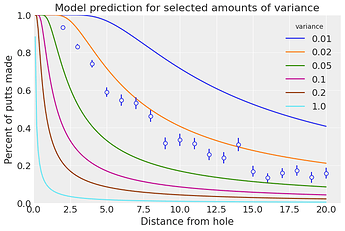
In the golf putting notebook, we define a forward_angle_model with xarray-einstats, then use it indistintively with 1d or 3d inputs for plotting and posterior predictive simulations. In the 1d input for plotting:

def forward_angle_model(variances_of_shot, t):
    norm_dist = XrContinuousRV(st.norm, 0, variances_of_shot)
    return 2 * norm_dist.cdf(np.arcsin((CUP_RADIUS - BALL_RADIUS) / t)) - 1

_, ax = plt.subplots()
t_ary = np.linspace(CUP_RADIUS - BALL_RADIUS, golf_data.distance.max(), 200)
t = xr.DataArray(t_ary, coords=[("distance", t_ary)])
var_shot_ary = [0.01, 0.02, 0.05, 0.1, 0.2, 1]
var_shot_plot = xr.DataArray(var_shot_ary, coords=[("variance", var_shot_ary)])

# both t and var_shot_plot are 1d DataArrays but with different dimension
# thus, the output is a 2d DataArray with the broadcasted dimensions
forward_angle_model(var_shot_plot, t).plot.line(hue="variance")

plot_golf_data(golf_data, ax=ax)  # This generates the scatter+error plot
ax.set_title("Model prediction for selected amounts of variance");


Bonus: I have also been looking into its potential to improve ArviZ using it as that would mean even better ArviZ-xarray integration, aka better scaling to posteriors with hundreds of variables/dimensions and much better scaling to models that don’t fit to memory. You can see some experiments on that and comparisons between xarray-einstats based rhat to the current ArviZ rhat in my GitHub.

7 Likes

Hi, thanks @OriolAbril,

This library will be really helpful for analyzing the posterior distributions of Bayesian models. Just wonder are you going to integrate any feature that supports Decision Analysis? Since after we build the model, we want deploy it, and make decisions from it :smile:

2 Likes

Not sure what you mean by Decision analysis in this context, could you give some examples of what you mean?

Hi, I totally agree with you on this point:

It is very common in Bayesian modeling to need to do further post-processing on the posterior samples in order to get meaningful and interpretable results, in many cases, these operations involve statistical or linear algebra.

Just want to add another popular case (in my opinion) is to do Decision Analysis with posterior distributions. I am no expert on this topic, but recently working on a similar problem in a real application.

The BDA3 book discussed Decision Analysis in chapter 9, which is referred in Stan’s document. I copy it here.

So basically, after the model has been built and we got the posterior inference. We may need to make some decisions from the inference result by doing some optimization on the posteriors with different options in a decision space.

Chapter 9 in BDA3 shows several examples how to do this, but there seems no available code examples yet (I searched for it before, but cannot find it).

One great example on Decision analysis using PyMC is in this blog post “Using Bayesian Decision Making to Optimize Supply Chains” by Thomas Wiecki & Ravin Kumar.

But I feel that it is kinds of difficult to work with posterior distributions to perform optimization. For example, in the above example (in cell 14), the authors only get some parts of posterior distribution (with [v:, 1]) for later optimization of the objective function.

supplier_yield_post_pred = pd.DataFrame({k: v[:, 1] for k, v in post_pred.items()})

I do not say this is wrong, but I wish that there is an easy way to work with posterior distributions to perform optimization in Decision Analysis.

So I think about a feature that could allow users to easily perform optimization with posterior distributions (xarray in this context). The optimization may use the scipy.optimize or use a optimization tool like Optuna.

It may difficult to do, but I think it could be a great feature to have :slight_smile:

2 Likes

You can already use xarray-einstats (and xarray alone in most cases) to compute the loss more easily, but the loss eventually returns a scalar value, so I don’t see how labeled and/or high dimensional data could help on that end.

Maybe we could update the post to pymc v4 and latest ArviZ+xarray. All the iterrows and conversions to datasets are not needed anymore. I think it would make a nice addition to pymc-examples. The loss function in the post is quite simple so there isn’t need for xarray-einstats really, xarray alone is enough.

And if you see examples of more complicated loss functions (i.e. requiring linear algebra or circmean if working with angles) it would also be nice to add a case study about this in xarray-einstats docs.

1 Like

I wrote a blog post on cmdstanpy and arviz integration that uses xarray-einstats for posterior predictive sampling:

Once you have an InferenceData object, nothing depends on coming from pymc, stan or even turing in julia so a large part of the post is also useful as an example of using xarray-einstats on pymc results.

3 Likes