I am trying to parameterize a model in the following way:
I have data that are from a series of experiments. The experiments should all give a consistent metric result (i.e. one of the parameters should be unimodal). But some of the experiments fail, in which case the data give no information about the result.
For each of the experiments, I want to average two models; a ‘passed experiment’ model, and a ‘failed experiment’ model. Both of these are different geometrical fits to the data, and the only parameter they share is the predicted data. For the ‘failed experiment’ model, the parameter of interest from the ‘passed experiment’ model is assigned a prior distribution, but the data don’t inform it at all.
Some of the experiments are ambiguous as to whether they passed or failed (either model could conceivably apply). I want to perform model averaging for each experiment. I then want to have the result from each experiment inform a top level parameter, so that they have common mean. Effectively I am weighting each experiment in a hierarchical model by how well they conform to the ‘pass’ model vs the ‘fail’ model.
Is there any way to parameterize a model like this (with the model comparison done at the individual level rather than the population level) in PyMC3? None of the examples I have seen currently do this.
I would introduce failure_rate as an additional parameter representing the prior probability of experimental failure. If you have repeated experiments, it can be treated hierarchically. Then the likelihood is a mixture model:
I would define P(X|\mathrm{fail}) as the expected likelihood of the data under the prior \int_\theta P(X|\theta)d\pi(\theta) which can be pre-computed. If you have more information about what failure modes might look like, you can use that too – ultimately your posterior estimates of r_\mathrm{fail} is heavily dependent on this term.
Firstly, how would you sum likelihoods like this in PyMC?
I can think maybe of creating a variable k~Bernoulli(r_{fail}) and then setting \theta=\theta_{pass}(1-k)+\theta_{fail}k but not certain if this is a valid way of doing this.
Secondly, what exactly is informing r_{fail} at the individual experiment level in this scenario? When I try doing simply the above, I just get the prior distribution. I assume that my predicted data for each of the models should be informing r_{fail} in some way, or that it would be my bayes factor for this?
Firstly, how would you sum likelihoods like this in PyMC?
Just make a deterministic node that tracks the likelihood. For instance, if you’ve got some regression model given a predicted value y_pred then you can do:
Now the likelihood will show up in the trace, so you can take np.log(np.mean(np.exp(tr['lik_y']))) as your Monte Carlo integrator. This converges quite nicely with number of data points (x axis):
Secondly, what exactly is informing r_{fail} at the individual experiment level in this scenario?
determining the population failure distribution. You can make this hierarchical if you’d like to estimate hyperparameters. Then you can tell from the posteriors which experiments are suspect:
while still retaining well-peaked posteriors for the parameters:
Thanks for the help with this. I would be interested in seeing other examples of this type of approach, e.g. if a textbook had examples of this it would be helpful. I’m assuming the thinking here is that although the data are best described by certain parameter values (leading to the posterior distribution), even that best set of parameter values isn’t particularly credible (marginal likelihood is small for that experiment).
Unfortunately my data in these case are vector data of different lengths for each experiment and running the model in this way seems to be inefficient. It’s a shame because it’s quite apparent that the model performs very poorly for some experiments just by looking at ppcs.
I’m thinking about using a more complex generative model to describe the ways in which the experiment fails, but the physics are complicated which may not make this any easier.
I’m assuming the thinking here is that although the data are best described by certain parameter values (leading to the posterior distribution), even that best set of parameter values isn’t particularly credible (marginal likelihood is small for that experiment).
Indeed. In effect you’d want to eliminate the failures for being far outside of the credible set. The approach taken here (a “flat” mixture model) is the simplest (and perhaps too simple) way to deal with anomalous points.
I have seen this termed as ‘Anomaly detection’:
or as ‘Outlier detection’:
and sometimes as ‘Robust Bayesian Inference’ (though this is a broad term which can mean robust to things besides outliers – such as misspecification).
This makes me wonder if there is a less computationally difficult way of achieving this. For my naive model, it’s actually quicker computationally to do a grid search than use an MCMC approach because there are many parameters which can be marginalized out analytically. It’s actually trivial to compute the marginal likelihood for each experiment through this method if I assume an uncertainty on the data points (I’ve used a value slightly higher than the measurement uncertainty is likely to be in order to capture experiments that may deviate slightly from physical assumptions but small enough that anything egregious isn’t credible). Would it be possible to use these calculated marginal likelihoods instead of the prior step in the notebook above? The hierarchical part of the model would still require MCMC as the number of experiments can be large.
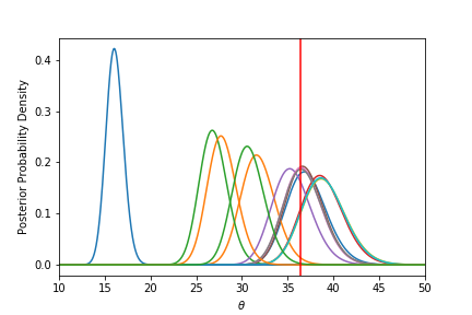
As an example, here are some data with their posterior probability density calculated using this method, with the red line being the target value. There are clearly some biased experiments in this case.
If I don’t normalize by the marginal likelihood, and instead just plot each experiment’s prior*likelihood, it becomes apparent that the biased values are extremely poorly served by this model(in some cases 40 orders of magnitude so). It seems fairly clear here that a hierarchical model with this weighting would give an unbiased result.
It’s also worth noting that the chance of failure at a population level for this experiment is not always low; in some cases the majority of experiments can be failures.
In writing this up, the structure of your data are a little bit unclear to me. The way I’m interpreting this is as a three-level model: Population (parameters that inform all experiments), experiment (some parameters are population-level, others are specific to an experiment), and trial (repeats of the same experiment). It’s not clear to me whether experiments can fail, or trials can fail, or whether “bad” experiments have a high failure rate for their nested trials.
I’m not sure what you mean by weight here.
Why not just use a hierarchical model? I know you specify “model averaging at individual level” in the title, but if you had (for the ith trial in the jth experiment):
While this is different from a marginal mixture model on the experiment level (which would really be tractable if you could parametrize the “failure” distribution); it does average trials to experiments, and experiments to population.
Sorry to cause confusion,
My data are vector data for individual experiments (the parameter of interest here is actually to do with the covariance of two measured data vectors, which is why many parameters can be analytically integrated out). I’m thinking of this as a two level hierarchy, some experiments don’t covary in a way that is meaningful for the parameter I am estimating. Therefore it’s the experiment that fails even though the individual measurements probably have small error.
If I use a hierarchical model where: P(\theta_{exp}|\theta_{pop}) \sim StudentT(\theta_{pop},\sigma,\nu)
Then the estimate of \theta_{pop} can be skewed by the biased \theta_{exp}.
By ‘weighting’, I mean I want to have the \theta_{exp} to have less influence over \theta_{pop} if they have lower marginal likelihood (i.e. they are unlikely to be telling us anything about the parameter because they conform so poorly to the model).
I suppose I could have \sigma (and/or \nu) be different for each experiment. This might deal with the problem if there are a small number of failed experiments, but not if there are a large number.
I think I’m still slightly confused by what exactly is meant by ‘expected likelihood of data under the prior’. To me this looks like the integral of the likelihood over the range of the prior, but that wouldn’t make sense as then you would always have P(X|\mathrm{fail}) >> P(X|\theta) and therefore a large r_{\mathrm{fail}}. It’s clear to me using a very simple grid search method with one parameter (i.e. in the case that I can get an analytical solution for the marginalized likelihood function for that parameter) that this should work if I had the correct P(X|\mathrm{fail}).
because you’ve integrated out your prior as opposed to choosing the point of highest density. This is a diversion from the real issue: you can pick values for failure rate r_\mathrm{fail} and data likelihoods P(X|\mathrm{fail}) that you think are reasonable; or you could even put priors over them (though you’d probably wind up with r_\mathrm{fail}=1 and P(X|\mathrm{fail})=1 if you’re not careful).
More generally, your estimates of \theta_{\mathrm{pop}} will always be influenced by failed experiments. Even under the mixture model you’d like, an experiment with the posterior distribution P(\mathrm{fail}|X) = 0.8 still has influence (albeit reduced) over the population estimate.
I suppose I could have σ (and/or ν) be different for each experiment.
This is precisely what the three-level model does, with an offset for experiment, and offset for trial within experiment. But If you don’t have replicates of experiments (or additional a-priori information about failure likelihoods) this doesn’t make sense: what’s to say that experiment 1 is (a priori) “more deviant” than experiment 5? Without repeats you can’t test whether experiment 1 is more variable than experiment 5, so parametrizing your model this way will only lead to overparametrization and divergences…
As a followup to this problem, I decided to use the linear mixture model. I’m still not entirely certain how to compute the expected likelihood of the data under the prior, but using a best guess for P(X|fail) appears to work quite well.
My individual experiments do not have repeated measurements in the sense that the same quantity is not measured twice under the same conditions. The experiments are measurements of two quantities under different temperature conditions, and the parameter of interest is the slope parameter of the line drawn by both quantities.
Physical or chemical processes that are not well understood cause the plots of experiment to be nonlinear. This can occur in a systematic way for a large proportion of experiments, leading to bias. I initially started predicting the value of the line with something analogous to a student’s t distribution, but this doesn’t work. As is quite apparent from the plots from two experiments below (best fitting line in green, data in red and blue), the ‘passed’ experiment is never going to have a posterior with 95% HPD overlap with the ‘failed’ experiment. Some examples are not so clear cut and it can be difficult to tell whether some experiments are biased so I want to use a probability of failure rather than a simple acceptance or rejection.
Unbiased experiment:
Biased experiment (note the x scale, estimate is ~4 times that of unbiased estimate):
The linear mixture model with an assumed small uncertainty works better in this case because the posterior for poor quality experiments becomes overwhelmed by the prior, which leads to a more unbiased estimate.
In brief, about 10% of the dataset has a “success” label at the beginning based on side information – in your case you have a pretty good idea which experiments obviously failed and which obviously succeeded. This enables the conditional model P(X|success) to be fit. The entire dataset is then assessed under the P(X|success) model, points below a threshold (or the lowest 1000) are treated as fail, and P(X|fail) is fit to these.
This is quite obviously non-Bayesian; as this is something like an E-M routine; though it works well in practice. It should be fairly straightforward to add priors P(success_i) and marginalize if you wanted to be truly Bayesian.