Multivariate Model outputting unusual intercept

bashj · March 16, 2021, 4:59am

Hello,

I have followed an article by Chad Scherrer on Bayesian Optimal Pricing and managed to get it to work well with my own data. I’ve also bound the beta variable to be a negative number. Using sales data for a single item, the model works as expected and the posterior prediction matches closely with the real data.

When I change the code going from examples provided in this forum on how to change it to a multivariate model, the values for beta match closely with the single item model, but the alpha is completely different, and if I feed these values into a formula to predict the quantity given a price, I get back values that are much larger. I am wanting to create a independent model so I can quickly get the elasticities for multiple items at the same time.

Single item model:

item_data = [{'p': 75.1, 'q': 54}, {'p': 78.64, 'q': 52}, {'p': 90.39, 'q': 21}, {'p': 96.06, 'q': 15}, {'p': 91.48, 'q': 18}, {'p': 89.76, 'q': 23}, {'p': 95.17, 'q': 15}, {'p': 86.36, 'q': 38}, {'p': 90.08, 'q': 25}, {'p': 93.89, 'q': 15}, {'p': 81.67, 'q': 44}, {'p': 83.6, 'q': 41}, {'p': 81.12, 'q': 33}, {'p': 82.81, 'q': 35}, {'p': 83.17, 'q': 29}, {'p': 88.87, 'q': 10}, {'p': 84.73, 'q': 16}, {'p': 82.1, 'q': 14}, {'p': 86.86, 'q': 20}, {'p': 94.4, 'q': 17}, {'p': 97.45, 'q': 24}, {'p': 89.41, 'q': 38}, {'p': 79.23, 'q': 132}, {'p': 73.53, 'q': 113}, {'p': 86.4, 'q': 44}, {'p': 78.98, 'q': 39}, {'p': 62.91, 'q': 78}, {'p': 62.92, 'q': 89}, {'p': 72.88, 'q': 130}, {'p': 71.8, 'q': 81}, {'p': 75.1, 'q': 53}, {'p': 75.75, 'q': 61}, {'p': 78.71, 'q': 35}, {'p': 78.94, 'q': 35}, {'p': 81.05, 'q': 55}, {'p': 64.71, 'q': 407}, {'p': 56.07, 'q': 277}, {'p': 64.14, 'q': 130}, {'p': 78.84, 'q': 82}, {'p': 82.47, 'q': 114}, {'p': 76.08, 'q': 72}, {'p': 86.98, 'q': 30}, {'p': 86.39, 'q': 37}, {'p': 82.04, 'q': 36}, {'p': 80.49, 'q': 36}, {'p': 82.78, 'q': 36}, {'p': 73.1, 'q': 42}, {'p': 76.94, 'q': 47}, {'p': 71.04, 'q': 59}, {'p': 80.27, 'q': 48}, {'p': 84.19, 'q': 40}]

items = pd.DataFrame(item_data)

with pm.Model() as m:
    a = pm.Cauchy('a',0,5)
    NegCauchy = pm.Bound(pm.Cauchy, lower=-np.inf, upper=0)
    b = NegCauchy('b',0,.5)
    logμ0 = a + b * (np.log(items.p) - np.log(items.p).mean())
    μ0 = pm.Deterministic('μ0',np.exp(logμ0))
    qval = pm.Poisson('q0',μ0,observed=items.q)

with m:
    t = pm.sample(1000, cores=1, tune=750)

plt.plot(t['a'],t['b'],'.',alpha=0.5);

Auto-assigning NUTS sampler...
Initializing NUTS using jitter+adapt_diag...
Sequential sampling (2 chains in 1 job)
NUTS: [b, a]
Sampling chain 0, 0 divergences: 100%|███████████████████████████████████████████| 1750/1750 [00:00<00:00, 1978.44it/s]
Sampling chain 1, 0 divergences: 100%|███████████████████████████████████████████| 1750/1750 [00:00<00:00, 2179.24it/s]

p = np.linspace(items.p.min() * .8, items.p.max() * 1.2, num=100)
np.exp(t.a + t.b * (np.log(p).reshape(-1,1) - np.log(items.p).mean()))

array([[ 965.68164247,  841.48493256, 1044.10041234, ..., 1023.8077616 ,
        1022.91339029, 1003.82476968],
       [ 889.34484971,  778.10209929,  959.9691476 , ...,  941.25641286,
         940.21155391,  922.88566178],
       [ 820.11200721,  720.38687373,  883.79282242, ...,  866.51496749,
         865.35144519,  849.60385152],
       ...,
       [   7.66359729,    8.46561696,    7.51595867, ...,    7.34453369,
           7.23680109,    7.20162925],
       [   7.4211787 ,    8.21076235,    7.273494  , ...,    7.10743644,
           7.00253458,    6.96914814],
       [   7.18787135,    7.9651006 ,    7.04029305, ...,    6.87940304,
           6.77724447,    6.74555433]])

Same item in a multivariate independent model:

items_data = [{'item': 0, 'p': 75.1, 'q': 54}, {'item': 1, 'p': 4.81, 'q': 38}, {'item': 0, 'p': 78.64, 'q': 52}, {'item': 1, 'p': 4.23, 'q': 39}, {'item': 0, 'p': 90.39, 'q': 21}, {'item': 1, 'p': 4.74, 'q': 26}, {'item': 0, 'p': 96.06, 'q': 15}, {'item': 1, 'p': 4.76, 'q': 33}, {'item': 0, 'p': 91.48, 'q': 18}, {'item': 1, 'p': 4.83, 'q': 44}, {'item': 0, 'p': 89.76, 'q': 23}, {'item': 1, 'p': 4.79, 'q': 56}, {'item': 0, 'p': 95.17, 'q': 15}, {'item': 1, 'p': 4.7, 'q': 47}, {'item': 0, 'p': 86.36, 'q': 38}, {'item': 1, 'p': 4.7, 'q': 57}, {'item': 0, 'p': 90.08, 'q': 25}, {'item': 1, 'p': 4.83, 'q': 65}, {'item': 0, 'p': 93.89, 'q': 15}, {'item': 1, 'p': 4.77, 'q': 71}, {'item': 0, 'p': 81.67, 'q': 44}, {'item': 1, 'p': 4.75, 'q': 66}, {'item': 0, 'p': 83.6, 'q': 41}, {'item': 1, 'p': 4.85, 'q': 65}, {'item': 0, 'p': 81.12, 'q': 33}, {'item': 1, 'p': 4.72, 'q': 66}, {'item': 0, 'p': 82.81, 'q': 35}, {'item': 1, 'p': 4.82, 'q': 68}, {'item': 0, 'p': 83.17, 'q': 29}, {'item': 1, 'p': 4.61, 'q': 75}, {'item': 0, 'p': 88.87, 'q': 10}, {'item': 1, 'p': 4.54, 'q': 64}, {'item': 0, 'p': 84.73, 'q': 16}, {'item': 1, 'p': 4.59, 'q': 86}, {'item': 0, 'p': 82.1, 'q': 14}, {'item': 1, 'p': 4.16, 'q': 87}, {'item': 0, 'p': 86.86, 'q': 20}, {'item': 1, 'p': 4.61, 'q': 72}, {'item': 0, 'p': 94.4, 'q': 17}, {'item': 1, 'p': 4.81, 'q': 67}, {'item': 0, 'p': 97.45, 'q': 24}, {'item': 1, 'p': 4.6, 'q': 53}, {'item': 0, 'p': 89.41, 'q': 38}, {'item': 1, 'p': 4.59, 'q': 60}, {'item': 0, 'p': 79.23, 'q': 132}, {'item': 1, 'p': 4.76, 'q': 58}, {'item': 0, 'p': 73.53, 'q': 113}, {'item': 1, 'p': 4.16, 'q': 55}, {'item': 0, 'p': 86.4, 'q': 44}, {'item': 1, 'p': 4.17, 'q': 60}, {'item': 0, 'p': 78.98, 'q': 39}, {'item': 1, 'p': 4.08, 'q': 44}, {'item': 0, 'p': 62.91, 'q': 78}, {'item': 1, 'p': 3.12, 'q': 49}, {'item': 0, 'p': 62.92, 'q': 89}, {'item': 1, 'p': 3.11, 'q': 68}, {'item': 0, 'p': 72.88, 'q': 130}, {'item': 1, 'p': 4.24, 'q': 61}, {'item': 0, 'p': 71.8, 'q': 81}, {'item': 1, 'p': 4.38, 'q': 41}, {'item': 0, 'p': 75.1, 'q': 53}, {'item': 1, 'p': 4.02, 'q': 57}, {'item': 0, 'p': 75.75, 'q': 61}, {'item': 1, 'p': 4.29, 'q': 49}, {'item': 0, 'p': 78.71, 'q': 35}, {'item': 1, 'p': 4.31, 'q': 58}, {'item': 0, 'p': 78.94, 'q': 35}, {'item': 1, 'p': 4.35, 'q': 41}, {'item': 0, 'p': 81.05, 'q': 55}, {'item': 1, 'p': 4.29, 'q': 47}, {'item': 0, 'p': 64.71, 'q': 407}, {'item': 1, 'p': 4.18, 'q': 69}, {'item': 0, 'p': 56.07, 'q': 277}, {'item': 1, 'p': 4.35, 'q': 54}, {'item': 0, 'p': 64.14, 'q': 130}, {'item': 1, 'p': 4.25, 'q': 54}, {'item': 0, 'p': 78.84, 'q': 82}, {'item': 1, 'p': 3.55, 'q': 65}, {'item': 0, 'p': 82.47, 'q': 114}, {'item': 1, 'p': 3.74, 'q': 76}, {'item': 0, 'p': 76.08, 'q': 72}, {'item': 1, 'p': 3.8, 'q': 67}, {'item': 0, 'p': 86.98, 'q': 30}, {'item': 1, 'p': 3.2, 'q': 57}, {'item': 0, 'p': 86.39, 'q': 37}, {'item': 1, 'p': 3.13, 'q': 67}, {'item': 0, 'p': 82.04, 'q': 36}, {'item': 1, 'p': 4.23, 'q': 53}, {'item': 0, 'p': 80.49, 'q': 36}, {'item': 1, 'p': 4.4, 'q': 49}, {'item': 0, 'p': 82.78, 'q': 36}, {'item': 1, 'p': 4.29, 'q': 36}, {'item': 0, 'p': 73.1, 'q': 42}, {'item': 1, 'p': 3.91, 'q': 56}, {'item': 0, 'p': 76.94, 'q': 47}, {'item': 1, 'p': 4.19, 'q': 49}, {'item': 0, 'p': 71.04, 'q': 59}, {'item': 1, 'p': 3.59, 'q': 58}, {'item': 0, 'p': 80.27, 'q': 48}, {'item': 1, 'p': 3.22, 'q': 78}, {'item': 0, 'p': 84.19, 'q': 40}, {'item': 1, 'p': 3.13, 'q': 56}]

items = pd.DataFrame(items_data)
n_items = items.item.nunique()

with pm.Model() as m:
    a = pm.Cauchy('a',0,5,shape=n_items)
    NegCauchy = pm.Bound(pm.Cauchy, lower=-np.inf, upper=0)
    b = NegCauchy('b',0,.5,shape=n_items)
    logμ0 = a[items.item] + b[items.item] * (np.log(items.p) - np.log(items.p).mean())
    μ0 = pm.Deterministic('μ0', np.exp(logμ0))
    qval = pm.Poisson('q0', μ0, observed=items.q)

with m:
    t = pm.sample(1000, cores=1, tune=750)

plt.plot(t['a'][:,0],t['b'][:,0],'.',alpha=0.5)

Auto-assigning NUTS sampler...
Initializing NUTS using jitter+adapt_diag...
Sequential sampling (2 chains in 1 job)
NUTS: [b, a]
Sampling chain 0, 41 divergences: 100%|███████████████████████████████████████████| 1750/1750 [00:08<00:00, 207.04it/s]
Sampling chain 1, 3 divergences: 100%|████████████████████████████████████████████| 1750/1750 [00:10<00:00, 165.94it/s]

There were 41 divergences after tuning. Increase `target_accept` or reparameterize.
The acceptance probability does not match the target. It is 0.6383162669604235, but should be close to 0.8. Try to increase the number of tuning steps.
There were 44 divergences after tuning. Increase `target_accept` or reparameterize.
The estimated number of effective samples is smaller than 200 for some parameters.

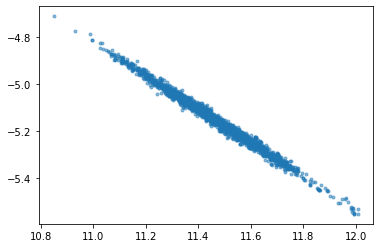
t.a[:, 0]

array([11.67, 11.65, 11.25, ..., 11.20, 11.33, 11.49])

t.b[:, 0]

array([-5.30, -5.28, -5.01, ..., -4.97, -5.07, -5.17])

pi = items.loc[items.item == 0].p
p = np.linspace(pi.min() * .9, pi.max() * 1.1, num=100)
np.exp(t.a[:,0] + t.b[:,0] * (np.log(p).reshape(-1,1) - np.log(pi).mean()))

array([[1380304.13, 1346367.87, 795723.19, ..., 742055.83, 881985.02,
        1085577.98],
       [1300175.60, 1268386.24, 751982.49, ..., 701535.30, 832900.29,
        1023999.46],
       [1225516.74, 1195717.65, 711094.97, ..., 663643.39, 787050.30,
        966543.95],
       ...,
       [27024.56, 26603.00, 19312.53, ..., 18471.94, 20412.33, 23316.39],
       [26264.13, 25856.15, 18798.38, ..., 17983.48, 19862.05, 22675.53],
       [25529.00, 25134.11, 18300.57, ..., 17510.45, 19329.44, 22055.58]])

ricardoV94 · March 16, 2021, 6:35am

I think in pm.Bound you should leave the unused bound as None instead of -np.inf.

Other than that your priors may be too broad when individual items are fit separately. If I get your scatter plot correctly, it seems a and b are highly correlated suggesting your data can be equally well explained by increasing one and decreasing the other or vice versa

chartl · March 16, 2021, 4:24pm

To expand on this: the system is under-determined. You have two parameters (intercept, slope) for every item, so 2N degrees of freedom for N items. You either need to reduce the degrees of freedom, or to regularize.

The latter is fairly straightforward: use a hierarchical model; and to get some decent regularization I’d suggest using a stringent error distribution like a Laplace. This would be something like

a_μ = pm.Cauchy('a_pop', 0, 5, shape=1)
b_μ = pm.Cauchy('b_pop', 0, 1, shape=1)  # we will use a mapping ([0, ∞) -> (-∞, 0])
a_offset = pm.Laplace('a_offset', 0, 1, shape=n_items)
b_offset = pm.Laplace('b_offset', 0, 1, shape=n_items)

a = pm.Deterministic('a', a_μ + a_offset)
b = pm.Deterministic('b', -tt.exp(b_μ + b_offset))

bashj · March 17, 2021, 1:50am

Thanks for the tips. So the model I thought was treating them as unrelated, but it was trying to find an unknown relationship between the items? Sorry, I’m not great at explaining what I was trying to do.

I found if I modify the following line of code, the item that had the unusual intercept was fixed in the multi-item model. The outputs from the single and multi models then match.

logμ0 = a[items.item] + b[items.item] * (np.log(items.p) - np.log(items.p).mean())

logμ0 = a[items.item] + b[items.item] * np.log(items.p)

chartl · March 17, 2021, 3:18pm

I was trying to explain the “tight” relationship between a and b that you plotted – and why there might be so many divergences.

If the divergences also went away after your switch, then the error was likely because the domain didn’t make sense. For instance, if all prices are >1 then all log-prices are positive; however, centering the log-prices (by subtrating the mean) will make some negative. Because b is sign-constrained this might be a problem.

bashj · March 17, 2021, 10:25pm

Thanks for explaining @chartl . I didn’t think of that!

Topic		Replies	Views
Zero One Inflated Beta Regression for an array of parameters Questions	10	538	June 22, 2023
Hierarchical Model with Multiple Predictors	5	770	August 15, 2023
Why does this Bayesian regression analysis fail? version agnostic	6	328	June 6, 2023
Can someone help me model this data...? version agnostic modeling	3	706	September 25, 2022
Bayesian Hierarchical Modelling with multiple timepoints for patients as an outcome Questions	2	337	February 11, 2021

Multivariate Model outputting unusual intercept

Related Topics