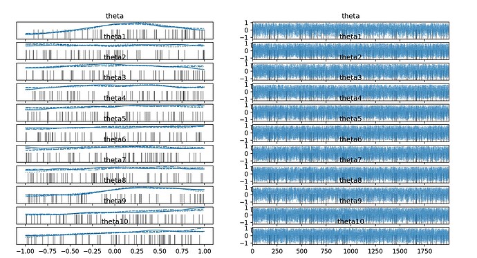
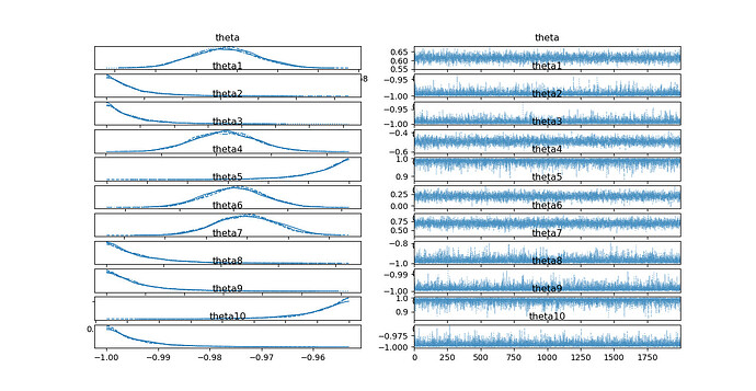
The standard deviation of posterior distribution remains the same compared to prior

[liu_liu]

Hi all, I am new to pymc and this is last step of my masters’s thesis. So whether this code worked is reallly important to me.

I am trying to fit parameters x in this form:

coefficients a is given as form of array.
I have a observed data like:
data = np.array([0.00882,0.02679, 0.04765, 0.07059, 0.09581,
0.11891, 0.14474, 0.17651, 0.19992, 0.22293, 0.2525, 0.27134,
0.29675, 0.32454, 0.34271, 0.36829, 0.38142, 0.40989])
every point in data has a linear regression mentioned above(different array a).
which means I need to find a set of parameters x to fit different points in data together best.

Now i = 11 I will set 11 priors, suppose they are all Normal~(0, 0.05)

my code is:

    with pm.Model() as model:

        theta = pm.Normal('theta',mu=0,sigma=0.1,shape=11)
        x=theta

        smiu = []

        for nm in range(len(A)):
            A1 = A[nm]
            sum1 = 0
            sum2 = 0
            sum3 =0
            former = 0
            for i in range(11):
                sum1 = x[i] * A1[i] + sum1  #
            d = 11
            for i in range(11):
                for j in range(i, 11):
                    sum2 = A1[d] * x[i] * x[j] + sum2
                    d = d + 1
            sum3 = math.log(curr_initial[nm]*1000) + sum1 + sum2  # *math.log(abs(curr_in))
            smiu.append(sum3)

        like = pm.Normal('like',mu=smiu, sigma=0.05,observed=data)
        trace = pm.sample(draws=2000,nuts_sampler="numpyro", progressbar=False,tune=1000)

        pm.sample_posterior_predictive(trace, extend_inferencedata=True)
        trace.posterior_predictive
        az.plot_ppc(trace, num_pp_samples=1000)

        az.plot_trace(trace)
        print(pm.summary(trace)[['mean', 'sd', 'mcse_mean', 'mcse_sd', 'r_hat']], 'trace')

        az.plot_posterior(trace)
        plt.show()

results are:

the result shows the standard deviation of posterior distribution nearly remains the same compared to prior. Is anything I did wrong? Is there any way to small the standard deviation?
I need the posterior distribution to be tall and thin.
I am using pymc5 python3.10 in windows.
the MWE is:
RS_bayesian.py (30.8 KB)

Thanks for any advice.

[cluhmann]

The first thing to note is that your trace is full of divergences (the black tick marks along the x-axis in the traceplot). So you should ignore the samples you are getting and figure out what is causing those divergences first. This notebook may be of some use.

[jessegrabowski]

I was thinking it’s an identification issue, and the divergences were just a symptom of that. I bet if we looked at pair plots, we’d see a bunch of straight lines.

From the equation it looks like a exponential-family GLM with interactions between the features (2nd summation term). In patsy, something like: y ~ a + b + c + d + a:b:c:d I think? But it’s unusual to define the coefficient of a * b as beta1 * beta2, since this isn’t going to be identifiable – that is, if the true effect is 1, there’s an infinite combination of beta1 * beta2 that equal 1, so the posterior geometry will be degenerate.

I also don’t think there’s any reason to think the effect of the interaction term would be the product of the effects? But I also don’t know anything about this model you’re working with.

[liu_liu]

Thanks for your answer.
So it’s impossible to get a correct posterior x y about this equation:
m=a + bx +cy+ dxx +eyy +fxy
a b c d e f m are known, set priors for x y ?

But I have to consider the multiplication of priors in my model .
Is there better way to deal with it?

[abang_tao]

Thanks, I will have a look at it!

[cluhmann]

I don’t think that’s the model you are currently specifying. Did you potentially mix up the predictors and the coefficients? As @jessegrabowski said, it looks like you are multiplying coefficients rather than predictors (e.g., e \cdot e \cdot y rather than e \cdot y \cdot y).

[liu_liu]

Hi, I’m sure I don’t mix up.

I use the above equation to replace a real model.
The model parameters is x(x_i, x_j), The coefficient is a(a_i, a_ij)
The coefficient a is fixed and calculated using sensitivity analysis based (SAB) method (page 4 of davis2003.pdf (1005.6 KB)) . I am sure this process is correct.
My purpose is to find a set of model parameters x to fit observed data (compared with the left of above equation) best to do uncertainty minimization and optimize the model parameters.

This method of parameter optimization seems to work correctly in queso (based on C and linux, My mentor did similar job using queso). The introduction of this library is queso .

so

@liu_liu

But I have to consider the multiplication of priors in my model

This also seems reasonable, so I am confused now.

@jessegrabowski

But it’s unusual to define the coefficient of a * b as beta1 * beta2, since this isn’t going to be identifiable – that is, if the true effect is 1, there’s an infinite combination of beta1 * beta2 that equal 1

[cluhmann]

Ok, I misinterpreted the mathematical specification (e.g., m=a + bx +cy+ dxx +eyy +fxy).

My suggestion is to begin by simulating data from a known model with known parameters and to simplify things down so that you only have a couple of predictors to begin with (e.g., something like m=a + bx +cy). Then, once you have that sampling (no divergences, successfully recovering true parameter values), then you can begin adding pieces back to the model (both the one used to simulate the data and the one used for inference). At some point, things will begin to break down and you should have a better sense of why. Like @jessegrabowski , I suspect that your data may not be well specified, and/or your priors may not play well with your (current) data.

[jessegrabowski]

From my side, I really don’t like the way to model uses loops and sums to build up your expression.

I would recommend multiplying the features in your dataframe together before you get into the PyMC model to make the x_i x_j combinations. Then you can write the PyMC model as just a single matrix multiplication, mu = X @ beta, with \beta = \begin{bmatrix} a_i \; | \;\text{vec}(a_{i,j}) \end{bmatrix} is a vector of all the parameters.

This would also make it easier to use named dims to make your outputs prettier.

Jesse

[liu_liu]

Hi Jesse
Matrix multiplication is a good suggestion, but how should I handle the term xixj? Should I set a separate prior for xi xj?

I don’t quite understand what you mean:

@jessegrabowski

I would recommend multiplying the features in your dataframe together before you get into the PyMC model to make the x_i x_jxixjx_i x_j combinations.

Will the use of loop and sum influence the result, or just influence the calculation speed or efficiency?

[jessegrabowski]

Loop and sum shouldn’t influence the result if you get everything right. But as you note it will be slower, and it also introduces the risk of getting something wrong. I am quite confident something is wrong is this model as-is.

I don’t really understand your setup well enough to make more specific recommendations. What is the connection between a_i and a_{i,j}? Or there is no connection? More concretely, if I compute \frac{\partial \eta}{\partial a_i}, do I get x_i, or is there also a cross term?

Also I would encourage you to refine the notation a bit. It’s quite confusing that you’re contrasting the words “parameters” and “coefficients” when these are typically used interchangeably. I guess you mean that the a terms are treated as data, whereas the x terms are estimated?

[liu_liu]

Ok.
I have a complex real model like: func(parameter_1,parameter_2…)
The inputs of model are parameters which are uncertain and I am trying to fix parameters’s values.
The output of model can be compared to experiment data(or observed data)

Since it’s very slow if I directly sample from my real model through blackbox likelihood function. (Using metropolis() gets incorrect result and using NUTS is too slow to get result)

Then I use a response surface to replace my real model. The response surface is like a second order polynomial, which can be determined using a simplified taylor expansion.

The left ln(eta) is the output of the model func(parameter_1,parameter_2…) .
The x_i and x_j… are the normalization forms of parameter_i , parameter_j and range [-1, 1].
The right a_0 is initial output which means all the priors(x) is 0
The a_i is first derivative of x_i.
The a_ij is the second derivative of x_j and x_j (partial differential).
I set uniform priors of x_i and x_j… and try to find a set of x fits observed data best.

[liu_liu]

Another question is about the likelihood:
like = pm.Normal(‘like’,mu=smiu, sigma=0.01,observed=data)
different sigma lead to different result, small sigma seems make the result better.
What could be the cause?

[ricardoV94]

Sounds like you have a very complex problem/model with too many things not working at the same time.

I would suggest simplifying the model (you can always just fit the mean) and building complexity incrementally.

This will allow you to have a better grasp of when things start to break down, and also increase the chance that someone can help here on the forum.

Regarding the sigma of the observed variable, it’s very uncommon to hard-code values since that’s rarely measured. Usually it’s given a more or less informative prior. This is something I would start playing with when writing the simplified models.

[liu_liu]

Thanks!
I don’t quite understand this:

@ricardoV94

you can always just fit the mean

cause my priors combine closely with each other(the xixj terms), so I think it’s hard for me to simplify the model. If I have y = a +bx +cy +dx^2 +ey^2 +fxy if I consider x and ignore y, when I add y will import new uncertainty of xy.

I define a specific value of sigma is because the observation values comes from an experiment referred in an essay and the essay shows their experiment uncertaity is 20%.

@ricardoV94

it’s very uncommon to hard-code values since that’s rarely measured.

[liu_liu]

I have another question these days.

For likelihood term,

logp += -np.sum((math.log(data[k]) - math.log(curr*0.0001))** 2.0) / (2.0 * sigma ** 2.0)

What is the impact of the magnitude of the likelihood function on the results, and can I multiply the likelihood function by a factor of 1000? The two variables I calculate in the likelihood function(data, curr) have real physical meaning, so I can modify their units.
When I multiply the likelihood function by 1000, the results seem good, the posteriors have distinct value, the occurrence of boundary values is acceptable because the parameters of the priors have physically meaningful constraints.

whereas they do not seem good without multiplication.

Both cases have uniform priors.

My question is: can I do the multiplication?
I know this can smaller the possibility of log likelihood term. But why does it seem to improve the results?
If I don’t multiply, the magnitude of the likelihood is- 0.05. If I do, the magnitude is -1e4 (*1000^2).

[cluhmann]

I don’t see this calculation in your model (but your model may have changed). Sampling should only ever consider the ratio between logp values (and the logps are unnormalized anyway, so their not even real probabilities), so their scale should matter except for some potential numerical stability issues. That being said, if you are calculating logps by hand, you have to make sure you are scaling the entire logp and not just some of the contributions to the total logp.